
This project (Github repository) is a python-based implementation of the methodologies presented in the paper Deep Smoothing of the Implied Volatility Surface by Ackerer et al (2020). The main idea is to use feedforward neural networks as a corrective tool to modify the prior models considered for volatility surfaces. By letting
\[\begin{equation} \omega(k,\tau; \theta):= \omega_{\text{prior}}(k,\tau;\theta_{prior})\cdot\omega_{\text{nn}}(k,\tau;\theta_{nn}), \end{equation}\]we enrich the space of parameters used for fitting the volatility surface. Here \(\omega\) is the implied variance and \(\theta_{\text{prior}}\) and \(\theta_{\text{nn}}\) are two disjoint set of parameters. Furthermore, to ensure our volatility surface is free of arbitrage, we could use the ideas by Roper (2010) which argues that if the following are satisfied then the call price surface is free of Calendar & Butterfly arbitrage resp.
\[\begin{align*} \ell_{cal}&:=\partial_\tau \omega(k,\tau) \geq 0 \\ \ell_{but}&:=\left(1-\frac{k\partial_k \omega(k,\tau)}{2\omega(k,\tau)} \right)^2-\frac{\partial_k \omega(k,\tau)}{4}\left(\frac{1}{\omega(k,\tau)}+0.25 \right)+\frac{\partial^2_{kk}\omega(k,\tau)}{2}\geq 0 \end{align*}\]Another condition required to guarantee a free-arbitrage VS is the large moneyness behaviour which states that \(\sigma^2(k,\tau)\) is linear for \(k\to \pm \infty\) for every \(\tau>0\). Roper achieves this by imposing \(\frac{\sigma^2(k,\tau)}{\vert k \vert}<2\) which in turn is achieved by minimizing the following
\[\begin{equation} \frac{\partial^2 \omega(k,\tau)}{\partial k \partial k} \end{equation}\]The above three constraints along with the prediction error are used to shape the loss function utilized in training the implied variance \(\omega\). For learning rate scheduling, a slightly different approach is taken compared to Ackerer et al. The following table summerizes the convergence techniques used for training:
| Checkpoint Interval | A checkpoint is set every 500 epochs. |
|---|---|
| Bad Initialization | After the first 4 checkpoints, if the best loss is not below 1, the model is reinitialized. |
| Learning Rate Adjustment | Every 4 checkpoints, if the best loss is not below 0.05, the learning rate is reset to its initial value. |
| Weights Perturbation | After each checkpoint, regardless of other conditions, the weights of the model are perturbed. This is to help escape local minima. |
| Divergence Handling (Bad Perturbation) | If the current loss is at least 10% worse than the best loss so far and > 0.1, and this occurs after the first checkpoint, the models are reloaded from the last saved state, and training continues from the last checkpoint with the best loss value. |
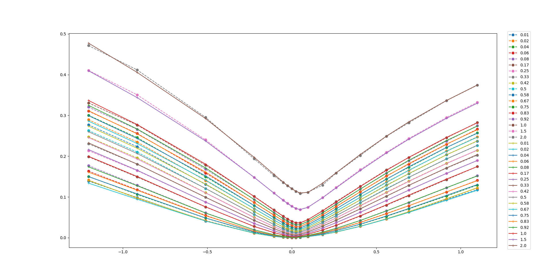
Numerical results show that the enhanced model, incorporating a neural network with the loss function \(\omega(k,\tau; \theta)\) with SSVI as prior, fits the Bates model data perfectly and produces an arbitrage-free volatility surface. The figure below shows how well the model fits the training data.
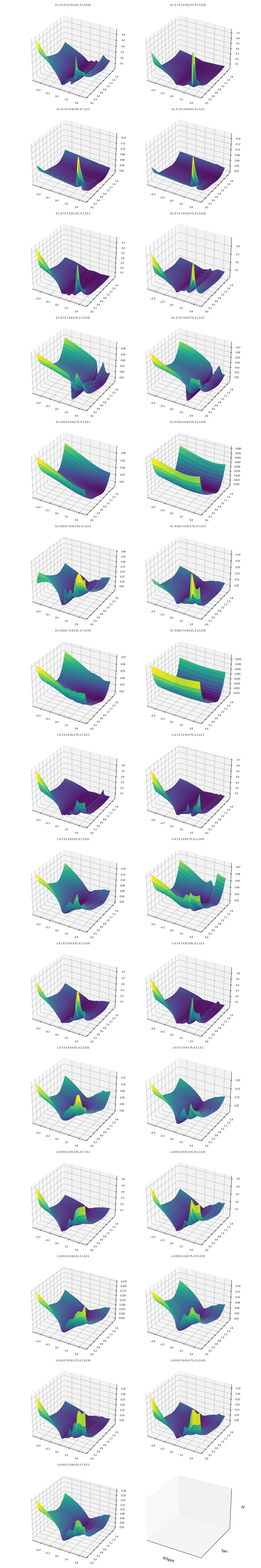
The figure below illustrates 29 trained implied volatility surfaces obtained using the deep smoothing algorithm for long term maturies obly i.e., \(\tau>\) 20 days. Different values for the Bates model parameters are used in each case. Displayed parameters are \(\alpha, \beta, \kappa, v0, \theta, \rho, \sigma, \lambda\) respectively. If you cannot guess the definition of these parameters see the technical report inside the github repository.
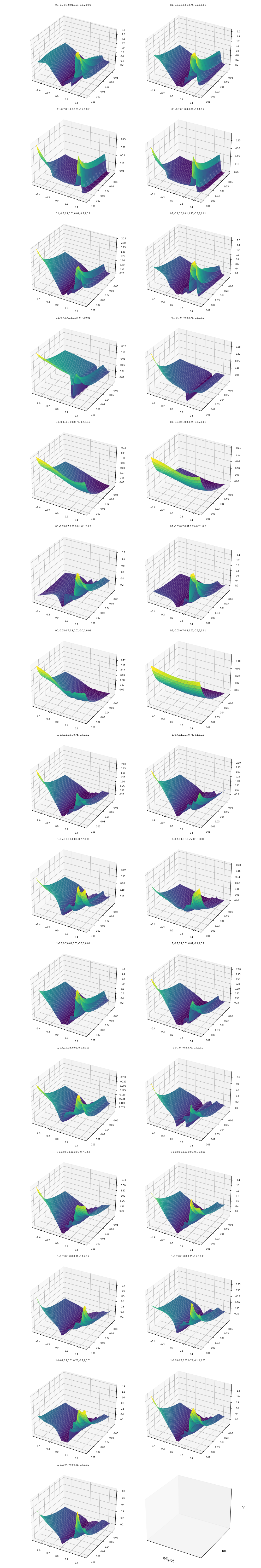
The figure below displays the same volatility surfaces for short term maturities i.e., \(\tau<=\) 20 days.
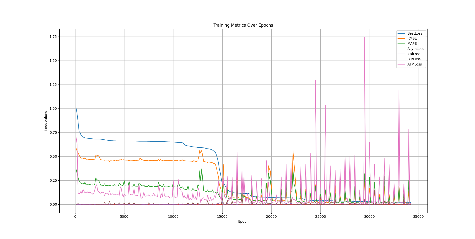
The following also is an example of the training trajectory where a feedforward neural network with 4 hidden layers, with 40 units in each layer.
See the technical report inside the Github repo for more details.