
Implementing Deep Smoothing for Implied Volatility Surfaces (IVS)
This project is a python-based implementation of the methodologies presented in the paper Deep Smoothing of the Implied Volatility Surface by Ackerer et al (2020) 1. A volatility surface is a representation of implied volatility across different strike prices and maturities, crucial for pricing and hedging options accurately. Ensuring the surface is arbitrage-free is essential to prevent inconsistencies that could lead to riskless profit opportunities, which would undermine the model’s reliability in real markets. You can find the code for this project here.
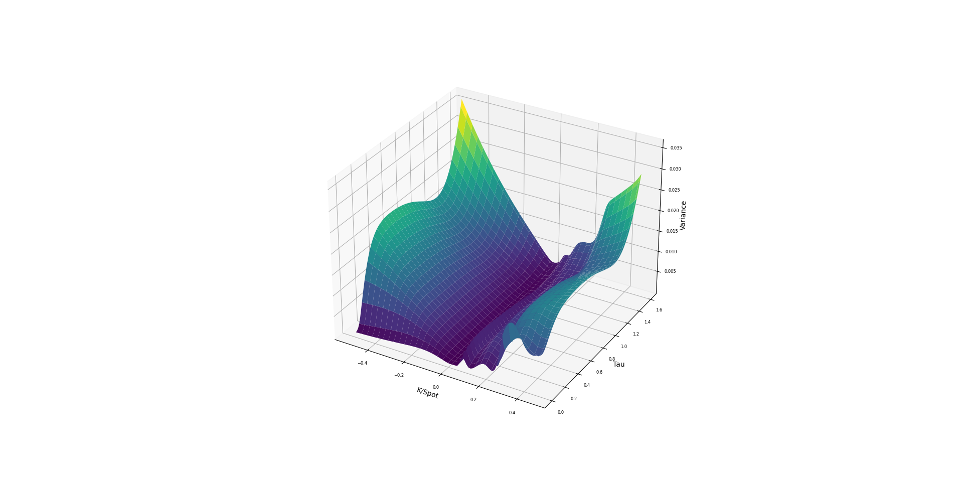
Table of Contents
- Introduction
- Notation and Initial Values
- Bates Model
- Loss Function
- ATM Total Variance
- Surface Stochastic Volatility Inspired (SSVI)
- Neural Network
- Convergence
- Results
- Final Remarks
- Appendix: Arb-Free Volatility Surfaces
- Bibtex
- References
Introduction
Deep smoothing focuses on applying deep learning methods to generate smooth, arbitrage-free implied volatility surfaces. For someone unfamiliar with quantitative finance, this problem can be summarized as follows: Imagine you are given a set of points \((k, \tau, iv)\) representing market data. These points form part of a 3D surface that we aim to construct with two key objectives:
- We need to fit the market data.
- We must ensure that the surface meets certain curvature properties. In quantitative finance, this means creating an arbitrage-free surface. Mathematically, this translates to minimizing a specified loss function across the entire surface.
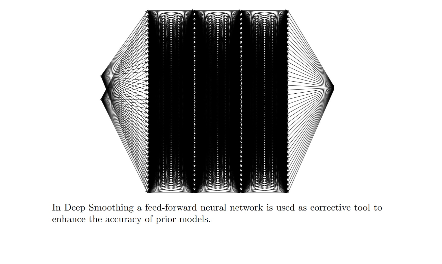
Deep smoothing’s main idea is to use feedforward neural networks as a corrective tool to modify the prior models considered for volatility surfaces (See 2 to learn more about prior models). By letting
\[\begin{equation} \omega(k,\tau; \theta):= \omega_{\text{prior}}(k,\tau;\theta_{prior})\cdot\omega_{\text{nn}}(k,\tau;\theta_{nn}), \end{equation}\]we enrich the space of parameters used for fitting the volatility surface. Here \(\omega\) is the implied variance and \(\theta_{\text{prior}}\) and \(\theta_{\text{nn}}\) are two disjoint set of parameters. The figure below displays a neural network with 4 hidden layers, each containing 40 units. The weights of this network are represented by \(\theta_{\text{nn}}\).
To ensure our volatility surface is free of arbitrage, we use the ideas from Arbitrage-free SVI Volatility Surfaces (2013) 2 where they argue that if the following are satisfied then the call price surface is free of Calendar & Butterfly arbitrage resp.
\[\begin{align*} \ell_{cal}&:=\partial_\tau \omega(k,\tau) \geq 0 \\ \ell_{but}&:=\left(1-\frac{k\partial_k \omega(k,\tau)}{2\omega(k,\tau)} \right)^2-\frac{\partial_k \omega(k,\tau)}{4}\left(\frac{1}{\omega(k,\tau)}+0.25 \right)+\frac{\partial^2_{kk}\omega(k,\tau)}{2}\geq 0 \end{align*}\]In this blog, we’ll walk through the main steps of the deep smoothing framework.
Notation and Initial Values
European call options with the following table of notation and values are used:
| Parameter | Value/Definition |
|---|---|
| Spot Price | spot = 1 |
| Strike | \(K\) |
| Interest Rate | rate \(= 0.0\) |
| Dividend Rate | \(q = 0.0\) |
| Forward Price | \(F_t\) |
| Forward Log Moneyness | \(k = \log \frac{K}{F_t}\) |
| Implied Volatility | \(\sigma(k, \tau)\) |
| Implied Variance | \(\omega(k, \tau) := \sigma(k, \tau)^2 \tau\) |
Table: Parameters and Definitions
Bates model
Bates dynamic is displayed below.
\[\begin{align*} \frac{dS_t}{S_t} &= (r - \delta) \, dt + \sqrt{V_t} \, dW_{1t} + dN_t \\ dV_t &= \kappa (\theta - V_t) \, dt + \sigma \sqrt{V_t} \, dW_{2t} \end{align*}\]\(dW_{1t}dW_{2t} = \rho dt\) and \(N_t\) is a compound Poisson process with intensity \(\lambda\) and independent jumps \(J\) with
\[\ln(1 + J) \sim \mathcal{N} \left( \ln(1 + \beta) - \frac{1}{2} \alpha^2, \alpha^2 \right)\]Characteristic Function
The characteristic function of the log-strike in the Bates model is given by:
\[\begin{align*} \phi(\tau,u) &= \exp\left(\tau \lambda\cdot \left(e^{-0.5\alpha^2u^2+iu\left(\ln(1+\beta)-0.5\alpha^2\right)}-1\right)\right) \\ &\cdot \exp\left(\frac{\kappa\theta \tau(\kappa-i\rho\sigma u)}{\sigma^2}+iu\tau(rate-\lambda\cdot \beta)+iu\cdot\log spot\right) \\ &\cdot \left(\cosh \frac{\gamma \tau}{2}+\frac{\kappa-i\rho\sigma u}{\gamma}\cdot\sinh \frac{\gamma \tau}{2}\right)^{-\frac{2\kappa \theta}{\sigma^2}} \\ &\cdot \exp\left(-\frac{(u^2+iu)v_0}{\gamma \coth \frac{\gamma \tau}{2}+\kappa-i\rho\sigma u}\right). \end{align*}\]We will use this characteristic function to price options in Bates model. To this end, we utilize FFTs.
Fast Fourier Transform
The option price calculation for the Bates model can be efficiently computed using an analytical formula that leverages FFT. Following Carr and Madan 3, we apply a smoothing technique to be able to compute the FFT integral. Recall that the option value is given by
\[C_\tau(k) = spot \cdot \Pi_1 - K e^{-rate \cdot \tau} \cdot \Pi_2\]where
\[\begin{align*} \Pi_1 &= \frac{1}{2} + \frac{1}{\pi} \int_0^\infty \text{Re} \left[ \frac{e^{-iu \ln(K)} \phi_\tau(u - i)}{iu \phi_\tau(-i)} \right] du \\ \Pi_2 &= \frac{1}{2} + \frac{1}{\pi} \int_0^\infty \text{Re} \left[ \frac{e^{-iu \ln(K)} \phi_\tau(u)}{iu} \right] du \end{align*}\]Since the integrand is singular at the required evaluation point \(u = 0\), FFT cannot be used to evaluate call price \(C_\tau(k)\). To offset this issue, we consider the modified call price \(c_\tau(k) := \exp(\alpha k) C_\tau(k)\) for \(\alpha > 0\). Denote the Fourier transform of \(c_\tau(k)\) by
\[\Psi_\tau(v) = \int_{-\infty}^{\infty} e^{ivk} c_\tau(k) \, dk \Rightarrow C_\tau(k) = \frac{\exp(-\alpha k)}{\pi} \int_0^\infty e^{-ivk} \Psi_{\tau}(v) \, dv\]It can be shown that
\[\Psi_\tau(v) = \frac{e^{-r \tau} \phi_\tau(v - (\alpha + 1)i)}{\alpha^2 + \alpha - v^2 + i(2\alpha + 1)v}\]We set up the FFT calculation as follows:
Log strike levels range from \(-b\) to \(b\) where \(b = \frac{Ndk}{2}\)
\(\Psi_\tau(u)\) is computed at the following \(v\) values: \(v_j = (j-1)du \text{ for } j = 1, \cdots, N\)
Option prices are computed at the following \(k\) values:
To apply FFT, we need to set \(dk \cdot du = \frac{2\pi}{N}\)
Simpson weights are used: \(3 + (-1)^j - \delta_{j-1} \text{ for } j = 1, \cdots, N\)
Having this setup ready, call prices are obtained as follows:
\[C(k_u) = \frac{\exp(-\alpha k_u)}{\pi} \sum_{j=1}^{N} e^{-i \frac{2\pi}{N} (j-1)(u-1)} e^{ibv_j} \Psi(v_j) \frac{\eta}{3} \left(3 + (-1)^j - \delta_{j-1}\right)\]The Python snippet below computes option prices using the Fast Fourier Transform (FFT). We use np.vectorize multiple times to vectorize the computations across various maturities and the corrective parameter, \(\alpha\).
def cf_bates(tau,u):


    u2, sigma2, alpha2, ju = u**2,sigma**2, alpha**2, 1j*u

    def log_phi_j():
        term1 = -0.5*u2*alpha2+ju*(np.log(1+beta)-0.5*alpha2)
        term2 = np.exp(term1)-1
        return tau*lam*term2

    a = kappa-ju*rho*sigma
    gamma = np.sqrt((sigma2)*(u2+ju)+a**2)
    b = 0.5*gamma*tau
    c = kappa*theta/(sigma2)

    coshb, sinhb = np.cosh(b), np.sinh(b)

    term1 = c*tau*a+ju*(tau*(rate-lam*beta)+np.log(spot))
    term2 = coshb+(a/gamma)*sinhb
    term3 = (u2+ju)*v0/(gamma*(coshb/sinhb)+a)
    res = log_phi_j()+term1-term3-2*c*np.log(term2)

    return np.exp(res)

N = 2**14  # number of knots for FFT
B = 1000  # integration limit

alpha_corrs = np.array([[[0.4,0.5,0.7,1]]])
n_a = alpha_corrs.shape[2]

du = B / N
u = np.array(np.arange(N)* du).reshape(1,-1,1)

w_fft = 3 + (-1) ** (np.arange(N) + 1)   # Simpson weights
w_fft[0] = 1 # [1, 4, 2, ..., 4, 2, 4]
dk = 2*np.pi/(du*N) # dk * du = 2pi/N
upper_b = N * dk / 2
lower_b = -upper_b
kus = lower_b + dk * np.arange(N)

taus_0_np = np.array(taus_0).reshape(-1,1,1) #n_t*1*1
w_fft = w_fft.reshape(1,-1,1) # 1*N*1
kus = kus.reshape(1,-1,1) # 1*N*1

cust_interp1d = lambda x,y: interp1d(x, y, kind='linear')
fn_vec = np.vectorize(cust_interp1d, signature='(n),(n)->()')

term1 = np.exp(-rate*taus_0_np)/(alpha_corrs**2+alpha_corrs-u**2+1j*(2*alpha_corrs+1)*u)
term2 = cf_bates(taus_0_np,u-(alpha_corrs+1)*1j)
mdfd_cf = term1*term2

integrand = np.exp(1j * upper_b * u)*mdfd_cf*w_fft* du / (3*np.pi)
vectorized_fft = np.vectorize(lambda i, j: fft(integrand[i,:, j]), signature='(),()->(n_k)')
tau_indices, corr_indices = np.indices((n_t, n_a))
integrand_fft = vectorized_fft(tau_indices, corr_indices).transpose(0, 2, 1)

Ck_u =np.exp(-alpha_corrs*kus)*np.real(integrand_fft )

f1 = Ck_u.transpose(1, 0, 2).reshape(N, -1)
fn = fn_vec([kus[0,:,0] for _ in range(n_t*n_a)],[f1[:,i] for i in range(n_t*n_a)])

spline = fn.reshape(n_t, n_a)
vectorized_spline = np.vectorize(lambda i, j, k: spline[i, j](ks[k]), signature='(),(),()->()')

tau_indices, corr_indices, ks_indices  = np.indices((n_t, n_a, n_k))
prices = vectorized_spline(tau_indices, corr_indices, ks_indices)
prices_ = prices.copy()
prices = np.median(prices,axis=1)
After computing prices, we use Quantlib library to obtain the volatility surface. We are now ready to explain the loss functions through which the arb-free conditions are enforced!
Loss Function
We define four different loss functions and construct the total loss function as a linear combination of these four, with coefficients being the penalty parameters. The first loss function is the prediction error, which is defined as below:
\[\begin{align*} \mathcal{L}_0(\theta) &= \sqrt{\frac{1}{\vert \mathcal{I}_0\vert} \sum_{(\sigma,k,\tau)\in \mathcal{I}_0} \left(\sigma-\sigma_\theta(k,\tau)\right)^2} + \frac{1}{\vert \mathcal{I}_0\vert} \sum_{(\sigma,k,\tau)\in \mathcal{I}_0} \frac{\left\vert \sigma - \sigma_\theta(k,\tau) \right\vert}{\sigma} \end{align*}\]Here, \(\mathcal{I}_0\) is the set of log-moneyness, implied volatility, and maturities for each observed market option. For future use, denote
\[\mathcal{T}_0 = \{ \tau:(0,\tau)\in \mathcal{I}_0 \}\]The other three loss functions are auxiliary, and consequently, we need to introduce auxiliary maturities and log-moneyness values. This ensures desired features for the constructed implied variance \(\omega\) across unobserved market data. Define
\[\begin{align*} \mathcal{T}_{aux} &= \left\{ \exp(x) : x \in \left[ \log\left(\frac{1}{365}\right), \max(\log(\tau_{\max}(\mathcal{T}_0) + 1))\right]_{100} \right\} \\ k_{aux} &= \left\{ x^3 : x \in \left[ -(-2k_{\min})^{1/3}, (2k_{\max})^{1/3} \right]_{100} \right\} \\ \mathcal{I}_{aux} &= \{(k, \tau) : k \in k_{aux}, \tau \in \mathcal{T}_{aux}\} \end{align*}\]where, for example, \(k_{\max} = k_{\max}(\mathcal{I}_0)\). Note that we consider more monyness around the money.
Calendar and Butterfly
Calendar and Butterfly loss functions are then defined as
\[\begin{align} \mathcal{L}_{cal}(\theta) &= \frac{1}{\vert \mathcal{I}_{Aux}\vert}\sum_{(k,t)\in \mathcal{I}_{Aux}} \max\left(0, -\ell_{cal}(k,\tau)\right) \\ \mathcal{L}_{but}(\theta) &= \frac{1}{\vert \mathcal{I}_{Aux}\vert}\sum_{(k,t)\in \mathcal{I}_{Aux}} \max\left(0, -\ell_{but}(k,\tau)\right) \end{align}\]Large Moneyness
For large moneyness behavior, we set
\[\mathcal{L}_{asym}(\theta) = \frac{1}{|\mathcal{I}_{asym}|} \sum_{(k, \tau) \in \mathcal{I}_{asym}} \left\vert \frac{\partial^2 \omega(k, \tau)}{\partial k \partial k} \right\vert\]where \(\mathcal{I}_{asym} = \left\{ (k, \tau) : k \in \{ 6k_{\min}, 4k_{\min}, 4k_{\max}, 6k_{\max} \}, \tau \in \mathcal{T}_{Aux} \right\}\)
Around the Money
We prefer that the prior component gives the best possible fit for ATM, while the neural network corrects the prior’s limitations for OTM. To this end, the following loss function is considered:
\[\mathcal{L}_{atm}(\theta) = \frac{1}{|\mathcal{I}_{\text{atm}}|} \left( \sum_{(k, \tau) \in \mathcal{I}_{\text{atm}}} (1 - \omega_{nn}(k, \tau; \theta_{nn}))^2 \right)^{1/2}\]Here \(\mathcal{I}_{\text{atm}} = \{(0, \tau) : \tau \in \mathcal{T}_{Aux}\}\).
Total Loss
The total loss function is constructed as follows:
\[\mathcal{L}_{Tot}(\theta) = \mathcal{L}_0(\theta) + \lambda_{but}\mathcal{L}_{but} + \lambda_{cal}\mathcal{L}_{cal} + \lambda_{atm}\mathcal{L}_{atm}\]Regularization parameters \(\lambda_{but}, \lambda_{cal}, \lambda_{atm}\) are tunable. In our experiments, we consider:
| Parameter | Value |
|---|---|
| \(\lambda_{atm}\) | 0.1 |
| \(\lambda_{but}\) | 4 |
| \(\lambda_{cal}\) | 4 |
Table: Loss Function Regularization Parameters
Python snippet below shows how loss function is computed given a pair of prior and neural network model i.e., \(\theta_{\text{prior}}\) and \(\theta_{nn}\), respectively.
def loss_butcal(model_prior, model_nn, ks, ts):

    kts = torch.stack((ks, ts), dim=1)
    output = model_prior(ks, ts)*model_nn(kts).squeeze(1)

    dw = torch.autograd.grad(outputs=output, inputs=[ks,ts], grad_outputs= torch.ones_like(output), create_graph=True, retain_graph=True)
    dwdk_,dwdtau_ = dw
    d2wdk_ = torch.autograd.grad(outputs=dwdk_, inputs=ks, grad_outputs=torch.ones_like(dwdk_), create_graph=True)[0]

    loss_but = relu(-((1-ks*dwdk_/(2*output))**2-(dwdk_/4)*(1/output+0.25)+d2wdk_/2)).mean()
    loss_cal = relu(-dwdtau_).mean()

    return loss_but, loss_cal

def loss_large_m(model_prior, model_nn, ks, ts):

    kts = torch.stack((ks,ts), dim=1)
    output = model_prior(ks, ts)*model_nn(kts).squeeze(1)
    dw= torch.autograd.grad(outputs=output, inputs=ks, grad_outputs=torch.ones_like(output), create_graph=True)
    dwdk = dw[0]
    grad_output_dwdk = torch.ones_like(dwdk)
    d2wdk = torch.autograd.grad(outputs=dwdk, inputs=ks, grad_outputs=grad_output_dwdk, create_graph=True)[0]
    loss_large_m = torch.abs(d2wdk).mean()

    return loss_large_m

def loss_atm(model_nn, ks, ts):

    kts = torch.stack((ks,ts), dim=1)
    output = model_nn(kts).squeeze(1)
    loss_atm = torch.sqrt(torch.pow(1-output,2).sum()/output.shape[0])

    return loss_atm

def loss_0(model_prior, model_nn):

    output = model_prior(df_torch_gpu[:,2], df_torch_gpu[:,3])*(model_nn(df_torch_gpu[:,2:4]).squeeze(1))
    sigma_theta = torch.sqrt(output/df_torch_gpu[:,3])
    temp = sigma_theta-df_torch_gpu[:,4]
    rmse = torch.sqrt(torch.pow(temp,2).mean())
    mape = (torch.abs(temp)/df_torch_gpu[:,4]).mean()

    return rmse, mape

def total_loss(model_prior, model_nn):

    ###########  Butterfly & Calendar Loss function ###############

    k_but_cal   = torch.tensor(ext(0,I_butcal), requires_grad=True).to(device)
    t_but_cal   = torch.tensor(ext(1,I_butcal), requires_grad=True).to(device)
    l_but, l_cal = loss_butcal(model_prior, model_nn,k_but_cal, t_but_cal)

    ###########  Large moneyness loss function ################

    k_large_m  = torch.tensor(ext(0,I_large_m), requires_grad=True).to(device)
    t_large_m  = torch.tensor(ext(1,I_large_m), requires_grad=True).to(device)
    l_large_m = loss_large_m(model_prior, model_nn, k_large_m, t_large_m)

    ###########  ATM loss function ###############

    k_atm = torch.tensor(ext(0,I_atm)).to(device)
    t_atm = torch.tensor(ext(1,I_atm)).to(device)
    l_atm = loss_atm(model_nn, k_atm, t_atm)

    ###########  L0 loss function ###############

    rmse, mape  = loss_0(model_prior, model_nn)

    ###########  Total loss ###############

    return rmse, mape, l_cal,l_but,l_large_m,l_atm
ATM Total Variance
The prior model is expected to provide a first-order approximation of the volatility surface, making it essential for the prior to accurately reproduce ATM (at-the-money) values. Since the ATM term structure is observable through market data for \(\tau \in \mathcal{T}_0\), we construct the ATM variance for each \(\tau \in \mathcal{T}_{aux}\) as described below.
Below are the steps to construct ATM variance:
- Step A: Ensure that \(\omega_{atm}(\tau_2) \geq \omega_{atm}(\tau_1)\) for every \(\tau_2 \geq \tau_1\). To achieve this, we solve the following optimization problem using quadratic programming (QP) with CVX:
Step B: Interpolate results from Step A using
scipywith a smoothing spline of degree 3Step C: Fit a degree-five polynomial to the result from Step B. This approach allows access to both \(\omega_{atm}(\tau)\) and its derivative \(\frac{\partial}{\partial \tau} \omega_{atm}(\tau)\) for each \(\tau \in \mathcal{T}_{aux}\), which is useful during the training process.
Python snippet below shows how ATM total variance is constructed.
import cvxpy as cv
from torch.autograd import Function
from scipy.optimize import curve_fit
from scipy.interpolate import UnivariateSpline

spot_variances = ... ## a numpy array containing atm variance
z = cv.Variable(len(spot_variances))
objective = cv.Minimize(cv.sum_squares(z - spot_variances))
constraints = [z[i] >= z[i-1]+1e-10 for i in range(1,len(spot_variances))]
prob = cv.Problem(objective, constraints)
prob.solve(verbose=False)
spot_variances_mdfd= z.value

spline_curve = UnivariateSpline(spot_taus, spot_variances_mdfd, k=5)
spline_curve.set_smoothing_factor(0.5)

def poly(x, *coeffs):
    return sum(c * x**i for i, c in enumerate(coeffs))

def poly_derivative(x, *coeffs):
    return sum(i * c * x**(i-1) for i, c in enumerate(coeffs) if i > 0)

degree = 5
popt, _ = curve_fit(poly, taus_aux,  spline_curve(taus_aux), p0=np.ones(degree+1))
popt_tensor = torch.tensor(popt).to(device)

# The at-the-money (ATM) variance and its derivatives are used as part of the neural network training process.
# To facilitate this, we define the following custom spline class, SPLFunction, which inherits from PyTorch's Function class.
class SPLFunction(Function):
    @staticmethod
    def forward(ctx, tau):
        ctx.save_for_backward(tau)
        return poly(tau,*popt_tensor)

    @staticmethod
    def backward(ctx, grad_output):
        tau, = ctx.saved_tensors
        grad_input = poly_derivative(tau,*popt_tensor)*grad_output
        return grad_input

def apply_spline(tau): return SPLFunction.apply(tau)
Surface Stochastic Volatility Inspired (SSVI)
The following version of the SSVI prior model (with power-law parameterization) has been used for the entire volatility surface.
\[\begin{align*} \omega_{\text{ssvi}}^{\text{prior}}(k, \tau) &= \frac{\omega_{\text{atm}}(\tau)}{2} \left( 1 + \rho \phi k + \sqrt{ \phi( k + \rho)^2 + 1 - \rho^2 } \right) \\ \phi &:= \phi(\omega_{\text{atm}}(\tau)) = \frac{\eta }{\omega_{\text{atm}}(\tau)^\gamma(1 + \omega_{\text{atm}}(\tau))^{1-\gamma}} \end{align*}\]Here \(\omega_{\text{atm}}(\tau)\) is the ATM term structure, and \(\rho\), \(\gamma\), and \(\eta\) are tunable parameters. In other words, we have:
\[\theta_{prior} = (\rho, \gamma, \eta)\]The Python snippet below shows how Wssvi is constructed. The function apply_spline, used here, is defined in the ATM Variance section above.
class Wssvi(nn.Module):
    def __init__(self):
        super().__init__()
        self.initialize_weights()

    def initialize_weights(self):

        self.gamma = nn.Parameter(torch.tensor(0.5))
        self.eta   = nn.Parameter(torch.tensor(1.0))
        self.rho   = nn.Parameter(torch.tensor(0.0))

    def forward(self, k, tau):

        t1 = apply_spline(tau)
        phi = self.eta*torch.pow(t1,-self.gamma**2)*torch.pow(1+t1,self.gamma**2-1)
        t2 = 1+self.rho*phi*k+torch.sqrt((phi*k+self.rho)**2+1-self.rho**2)
        return t1*t2/2
Neural Network
For the feed-forward neural network, we use 4 layers, each with 40 units. The model is trained using the Adam optimizer in conjunction with the optim.lr_scheduler.ReduceLROnPlateau scheduler. To escape local minima, we reinitialize weights when necessary. See the Convergence section below for more details. The Python snippet below provides the code for constructing the neural network class.
class NN(nn.Module):
    def __init__(self, input_size, hidden_sizes, output_size):
        super().__init__()
        layers = []
        in_size = input_size
        for hidden_size in hidden_sizes:

            layers.append(nn.Linear(in_size, hidden_size).to(torch.float64))
            layers.append(nn.Softplus())
            in_size = hidden_size
        layers.append(nn.Linear(in_size, output_size).to(torch.float64))
        layers.append(oneplustanh())
        self.layers = nn.ModuleList(layers)
        self.network = nn.Sequential(*layers)
        self.initialize_weights()

    def initialize_weights(self):
        for layer in self.layers:
            if isinstance(layer, nn.Linear):
                n_in = layer.in_features
                n_out = layer.out_features
                std = (1 / (n_in + n_out))**0.5
                nn.init.normal_(layer.weight, mean=0, std=std)
                nn.init.normal_(layer.bias, mean=0, std=std)

    def forward(self, x):
        # return torch.tensor([[1]]).to(device)
        return self.network(x)

def reinitialize_model(model,weight_init,scheduler_class, scheduler_args, lr=learning_rate):

    if weight_init:
        model.initialize_weights()

    optimizer = optim.Adam(model.parameters(), lr=lr)
    scheduler = scheduler_class(optimizer, **scheduler_args)
    return optimizer, scheduler
Convergence
For learning rate scheduling, a slightly different approach is taken compared to Ackerer et al. The following table summerizes the convergence techniques used for training:
| Checkpoint Interval | A checkpoint is set every 500 epochs. |
|---|---|
| Bad Initialization | After the first 4 checkpoints, if the best loss is not below 1, the model is reinitialized. |
| Learning Rate Adjustment | Every 4 checkpoints, if the best loss is not below 0.05, the learning rate is reset to its initial value. |
| Weights Perturbation | After each checkpoint, regardless of other conditions, the weights of the model are perturbed. This is to help escape local minima. |
| Divergence Handling (Bad Perturbation) | If the current loss is at least 10% worse than the best loss so far and > 0.1, and this occurs after the first checkpoint, the models are reloaded from the last saved state, and training continues from the last checkpoint with the best loss value. |
Results
We have two kinds of training: training a reference model and training models using the reference model for initialization. Training the reference model takes significantly more time, whereas training other models based on it takes much less time. The following table shows the parameter values of the reference model as well as an example of those of a subsequent model trained based on the reference model. It is emphasized that training the subsequent model is much faster.
| Parameter | Reference Model | Subsequent Model (Ex) |
|---|---|---|
| \(\alpha\) | 0.7 | 0.5 |
| \(\beta\) | -0.03 | -0.04 |
| \(\kappa\) | 0.5 | 0.4 |
| \(v_0\) | 0.01 | 0.02 |
| \(\theta\) | 0.0625 | 0.05 |
| \(\rho\) | -0.75 | -0.65 |
| \(\sigma\) | 1 | 0.8 |
| \(\lambda\) | 0.2 | 0.3 |
Table: Parameter Values
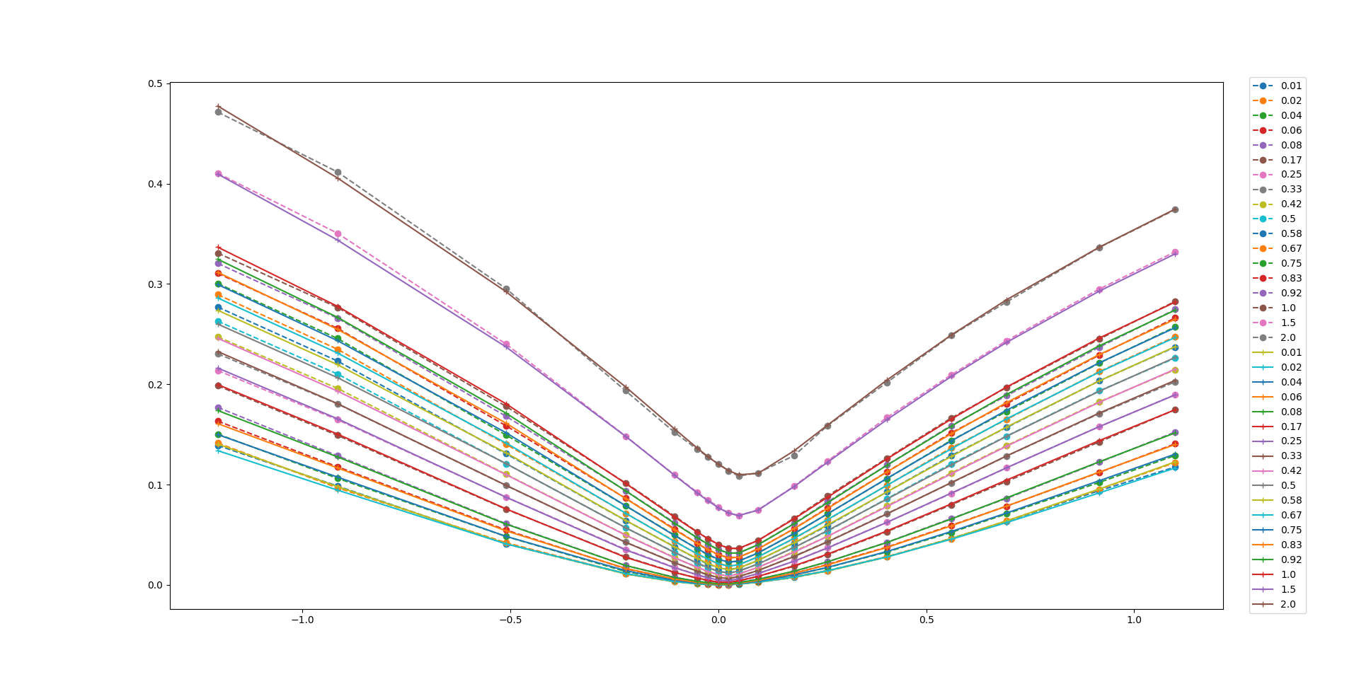
Numerical results show that the enhanced model, incorporating a neural network with the loss function \(\omega(k,\tau; \theta)\) with SSVI as prior, fits the Bates model data perfectly and produces an arbitrage-free volatility surface. The figure below shows how well the model fits the training data.
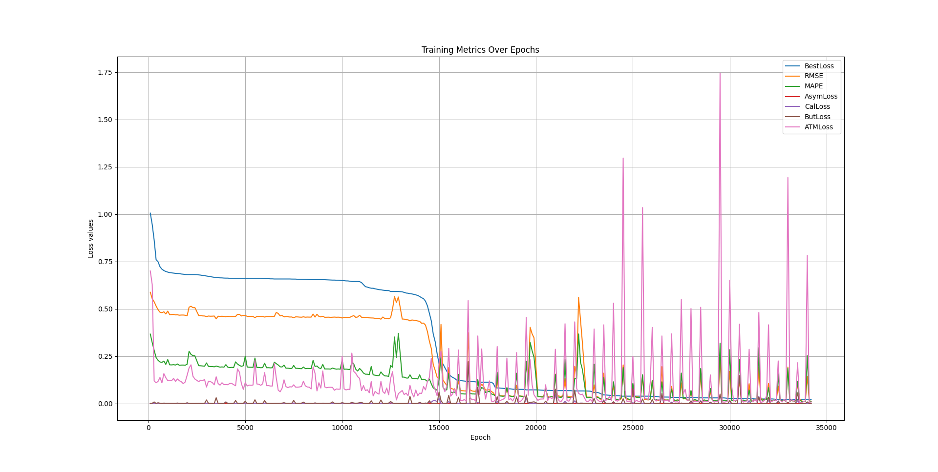
The following also is an example of the training trajectory where a feedforward neural network with 4 hidden layers, with 40 units in each layer.
Final Remarks
Several numerical experiments are still to be conducted using the project code. These experiments include applying deep smoothing to real market data rather than synthetic data, performing backtesting, examining W-shaped smile patterns, investigating different sizes for neural network layers, and comparing results with a stand-alone prior (which can be easily implemented by setting the neural network’s forward pass output to 1). We encourage interested readers to explore these avenues further.
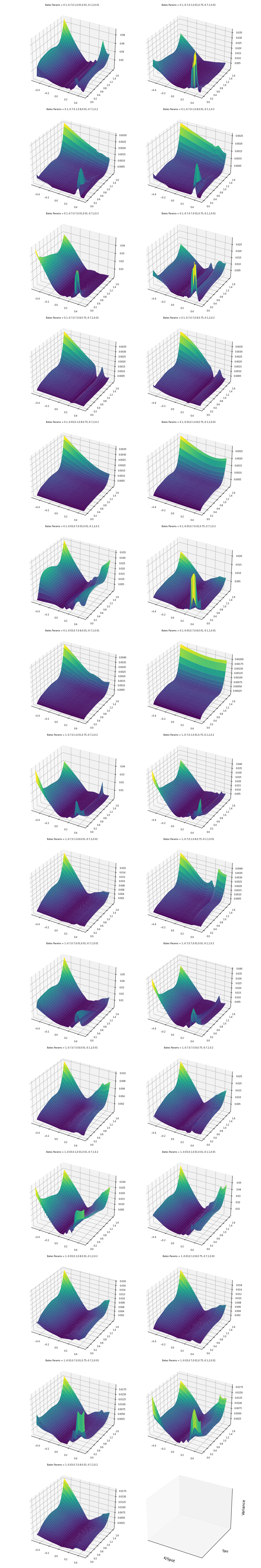
Appendix: Arb-Free Volatility Surfaces
The figure below illustrates 29 trained implied variance surfaces obtained using the deep smoothing algorithm. Different values for the Bates model parameters are used in each case. Displayed parameters are \(\alpha, \beta, \kappa, v_0, \theta, \rho, \sigma, \lambda\) respectively. .
Bibtex
@misc{baghal2024implementing,
  title={Implementing Deep Smoothing for Implied Volatility Surfaces (IVS)},
  author={Baghal, Sina},
  journal={https://sinabaghal.github.io/deepsmoothing/},
  url={https://sinabaghal.github.io/deepsmoothing/},
  year={2024}
}
References
Ackerer, D., Tagasovska, N., & Vatter, T. (2020). Deep Smoothing of the Implied Volatility Surface. arXiv:1906.05065 ↩
Gatheral, J., Jacquier, A. (2013). Arbitrage-free SVI volatility surfaces. arXiv:1204.0646 ↩ ↩2
Carr, P., Madan, D. (2001). Option valuation using the fast Fourier transform. CarrMadan.pdf ↩