Implied Volatility

Implied volatility is a crucial concept in financial markets, reflecting the market’s forecast of a security’s price fluctuation over a specific period. It is derived from the market price of an option and represents the volatility that, when input into the Black-Scholes model, yields the observed market price. Implied volatility is a key metric for traders and investors in the assessment of market expectations and the pricing of options. Recall the Black-Scholes formula:

\[c(\sigma) = SN(d_+)-Ke^{-r\tau}N(d_-) \text{ where } d_{\pm} = \tfrac{1}{\sigma\sqrt{\tau}}[\log \tfrac{S}{K}+(r\pm\tfrac{\sigma^2}{2})\tau]\]

\(c(\sigma), S, K, r, \tau\) are market observed data and solving this equation for \(\sigma\) provides the implied volatility (IV). It is emphasized that solving this equation is numerically challenging as it involves the Gaussian CDF which levels off rapidly both for positive and negative values. Due to this fact, any use of Newton root finding algorithm requires careful consideration as for the initialization.

Below, I provide a code in Python that calculates IV for index options (prices from CBOE.com). This code is not optimized and for clarity it’s kept as-is. It solves for IV using a combination of bisection and Newton root finding algorithm. Option prices outside of the allowable range within the Black-Scholes framework are discarded.

import numpy as np ; import pandas as pd 
import scipy.stats as st; import scipy.optimize as opt


# Index option data is downloaded from CBOE.com.
options = pd.read_csv('data/eod_marking_prices_list.csv')
spx_options = options[options.underlying_symbol == '^SPX']
rates = pd.read_csv('data/FEDFUNDS.csv')
r0 = rates[rates['DATE'] == '2024-05-01'].FEDFUNDS.values[0]/100 # Interest rate

entries = []
for row_cnt in range(spx_options.shape[0]):

    # print('Row number  = ', row_cnt)
    entry = {}
    row = spx_options.iloc[row_cnt,:]
    S = row.call_underlying_value  # Today's stock price
    K =  row.strike # Strike price
    tau = row.DTE/252 # time to maturity

    ## It'd be better if midpoint of ask and bid price is used even though
    # that's not guaranteed to be arbitrage free. 
    market_price = row.call_final_indicative_ask # Market call option price
    zeta = (S/K)*np.exp(r0*tau) ## forward moneyess (or its inverse)

    d1 = lambda sigma: (np.log(S / K) + (r0 + 0.5 * sigma ** 2) * tau)/(sigma * np.sqrt(tau))
    d2 = lambda sigma: (np.log(S / K) + (r0 - 0.5 * sigma ** 2) * tau) / (sigma * np.sqrt(tau))

    def call_price(sigma):
    # Compute call option price as a function of sigma.  
    # Since vega is positive, call_price(sigma) is increasing w.r.t. sigma.

        if sigma >0:
            return (S * st.norm.cdf(d1(sigma)) - K * np.exp(-r0 * tau) * st.norm.cdf(d2(sigma)))
        elif sigma == 0:
            if zeta>1:
                return S - K * np.exp(-r0 * tau) 
            elif zeta ==1:
                return 0.5*(S - K * np.exp(-r0 * tau))
            else:
                return 0

    call_function      = lambda sigma: call_price(sigma) - market_price
    # import pdb; pdb.set_trace()
    if call_function(0) > 0 : 
        # i.e., market price is outside of allowable range and data is discarded
        continue
    
    # upper_bound = 2*np.sqrt(np.abs(np.log(zeta)))
    ## Next, we obtain an interval which contains IV.
    upper_bound = 0.4
    while call_function(upper_bound) < 0: 
        upper_bound =  2*upper_bound
    while call_function(upper_bound) >0:
        # import pdb; pdb.set_trace()
        if call_function( 0.5*upper_bound) >0:
            upper_bound =  0.5*upper_bound
        else: 
            lower_bound = 0.5*upper_bound
            break 

    assert(call_function(lower_bound)<0);  assert(call_function(upper_bound)>0)  
    # Apply Newton's root finding algorithm using the midpoint of the interval above.
    init_newton = (lower_bound+upper_bound)/2

    newton_sol = opt.newton(call_function,  init_newton, tol=1e-10, maxiter=1000, disp=True, full_output=True)
    implied_vol = newton_sol[1].root
    error = np.abs(call_price(implied_vol) - market_price)
    
    entry['K'], entry['S'], entry['Moneyness'], entry['tau'], entry['market_price'],entry['IV'],entry['error'] = \
    K,S, S/K, tau, market_price, implied_vol,error

    entries.append(entry)

df = pd.DataFrame(entries)
df.to_csv('result_22June_V1.csv')

Fixing time to maturity \(\tau\) and ploting IV against strike, the volatility smile is obtained.

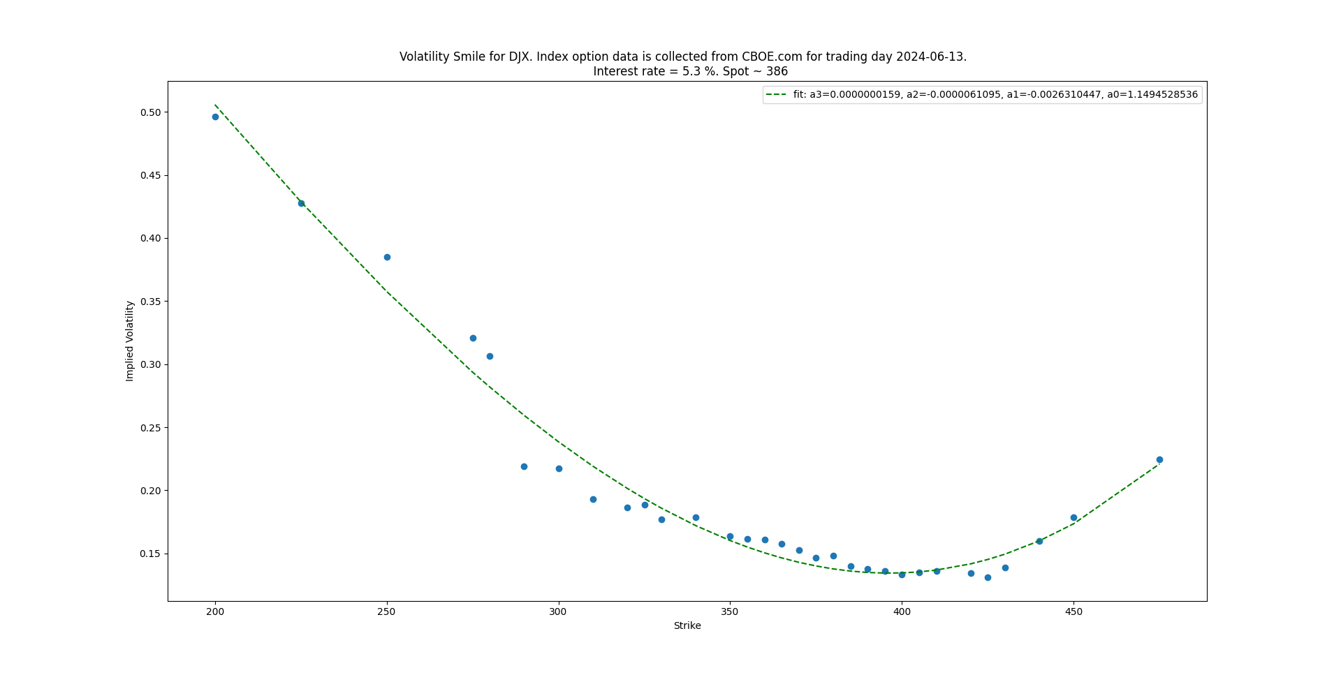
Here is also the curve-fitting code:

df_tau = df[df.tau == df.iloc[0,:].tau]
def func(x, a3,a2,a1,a0):
    return a3 * x**3+a2*x**2+a1*x + a0

popt, pcov = curve_fit(func, df_tau.K,  df_tau.IV)
plt.plot(df_tau.K, func(df_tau.K, *popt), 'g--',
         label='fit: a3=%5.10f, a2=%5.10f, a1=%5.10f, a0=%5.10f' % tuple(popt))
# plt details omitted for brevity

Sina Baghal