Solving Pasur Using GPU-Accelerated CFR
🚧🚧🚧🚧 Under Construction 🚧🚧🚧🚧
This repository is dedicated to the paper Solving Pasur Using GPU-Accelerated Counterfactual Regret Minimization. You can find the code for this project here.
The main aim of this work is to train an algorithm that can play the card game Pasur optimally. The contents of this webpage provide only a summary of what is discussed in the paper, with many details omitted. For the complete discussion, please refer to the paper linked above.
Table of Contents
Counterfactual Regret Minimization
I begin by explaining Counterfactual Regret Minimization (CFR). Suppose we have two players, Alex and Bob, who are playing a game and the corresponding game tree is shown here. The goal of the CFR algorithm is to find an optimal strategy for both players.
By strategy, we mean a probability distribution over the possible actions at each node of the tree. For example, at the node denoted by B in the figure below, Bob has two actions where based on his current strategy, one action may be chosen with probability 20% (as shown) and the other with probability 80%.
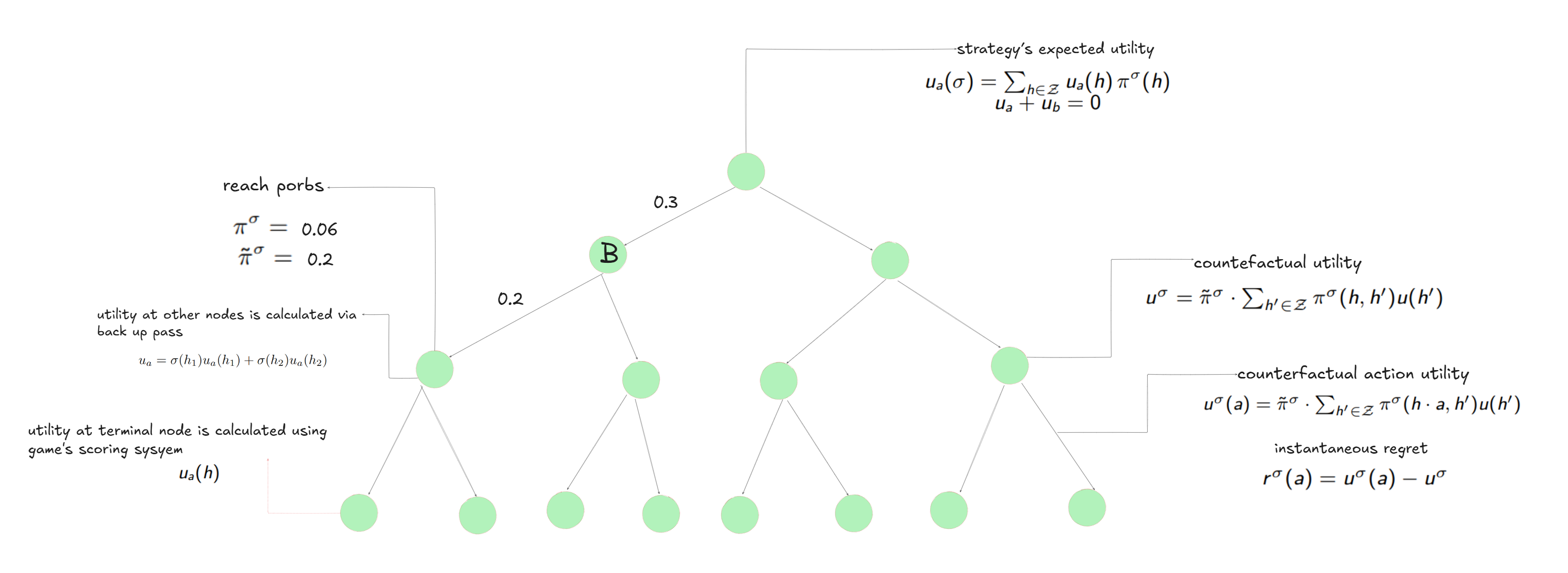
Utilities at terminal nodes are defined naturally via the game’s scoring system. Utilities at other nodes is calculated via a backup pass. Notice that since we are in a zero-sum setting, the utilities of Alex and Bob always sum to zero at each node of the game tree. In other words, \(u_a\) plus \(u_b\) equals zero.
Now, we are looking to find an optimal strategy for both players. Here by “optimal strategy,” we mean a Nash Equilibrium. This is a pair of strategies where no player can improve their payoff by changing their own strategy while the other keeps theirs fixed.

Next, we define something called instantaneous regret for each action. Instantaneous regret is defined as the counterfactual utility of that action minus the counterfactual utility of the current node. The definitions are written here. Counterfactual utility of a node is the probability of reaching that node—assuming the current player has purposefully reached that node—multiplied by the expected utility if play continues from that point. Counterfactual utility of an action is defined in the same way.
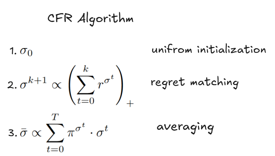
CFR is a classic algorithm that provably converges to this Nash Equilibrium. The idea of CFR is straightforward. We start with a uniform strategy, meaning each action is taken with equal probability. For example, if there are two actions, each one is chosen with probability 50%. At each iteration, we compute these instantaneous regrets for all nodes and store them. We then update the strategy by assigning probabilities to actions in proportion to the sum of all accumulated regrets up to the current iteration. Finally, the output of CFR is the weighted average of all strategies observed so far, where the weights are given by the reach probabilities.
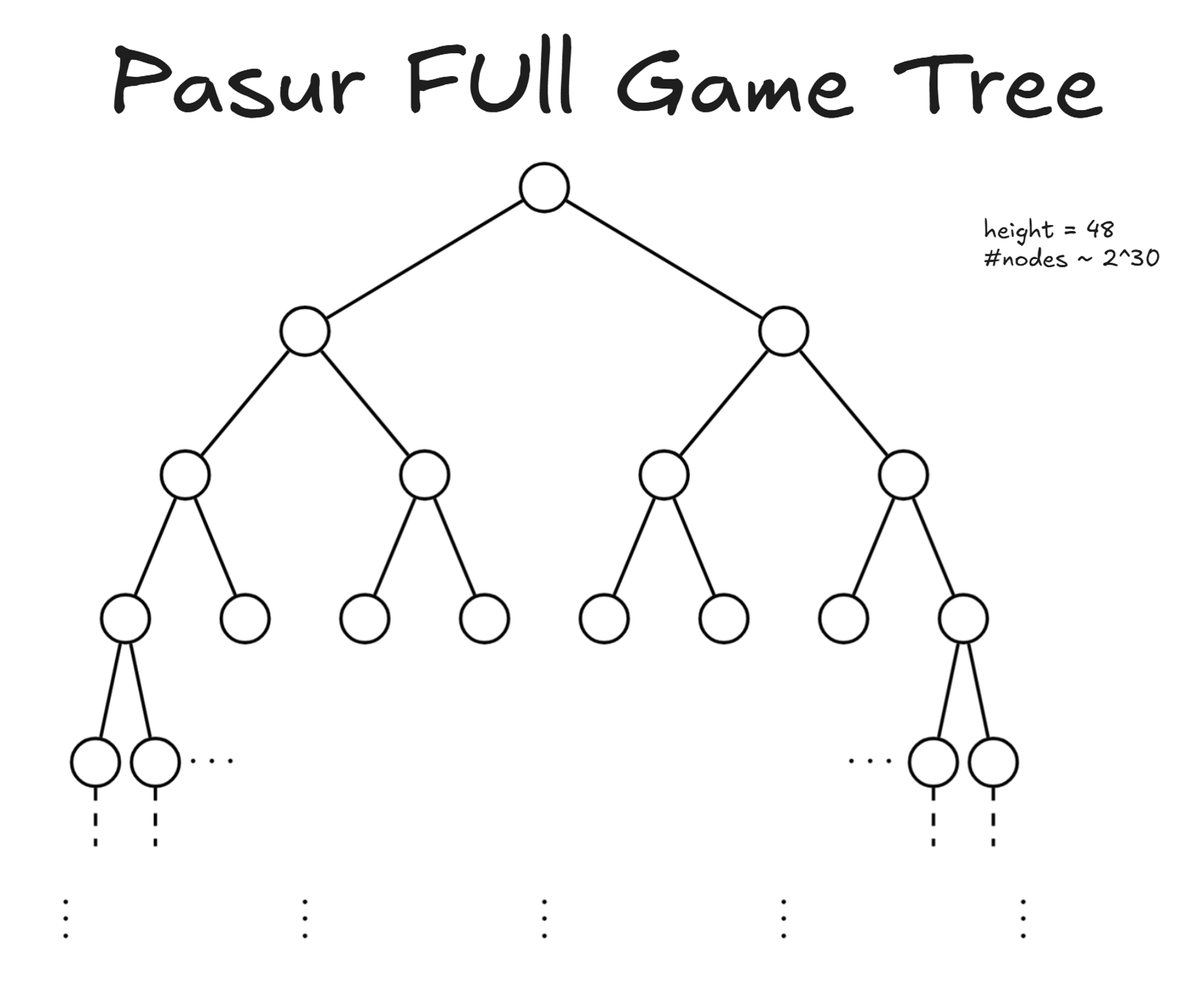
The aim of this work is to run CFR on the Pasur game tree, which has a height of 48 and an average size of about 2 to the power of 30 nodes.
Pasur
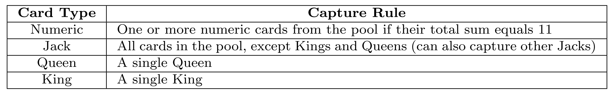
Pasur is played in 6 rounds, and in each round each player is dealt 4 cards, which they play sequentially over 4 turns, taking turns one after another. At each turn, a player places a card face up and either lays it in the pool or collects it along with some other pool cards, according to the rule shown in this table. Figure below shows an example of the first turn by Alex and Bob.
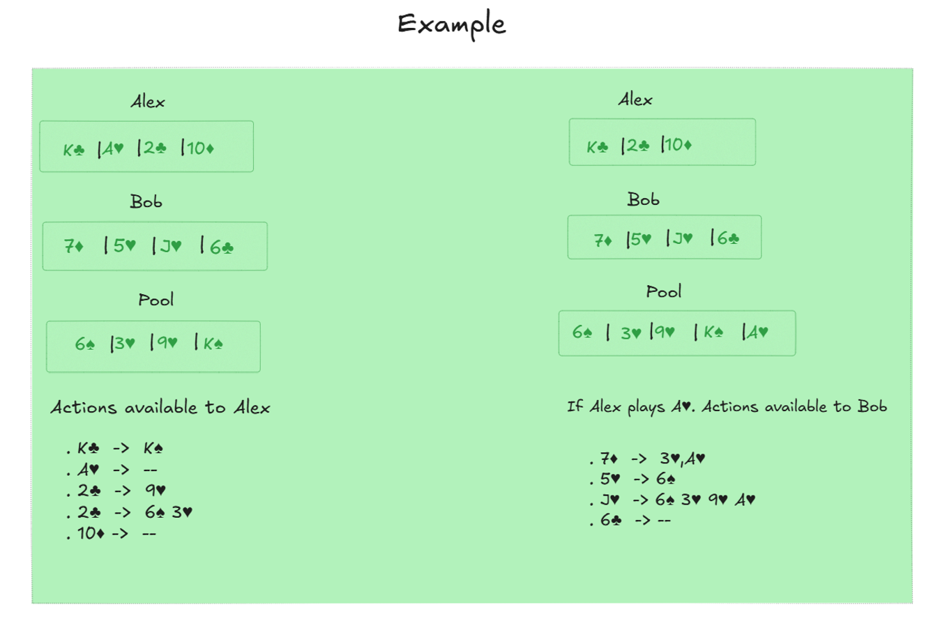
Let me explain the rule and scoring system in more detail. If the played card is numeric, it can collect any subset of cards whose values add up to 11. If it is a Jack, it can collect all cards in the pool except for Kings and Queens. If it is a King, it can only collect a single King, and if it is a Queen, it can only collect a single Queen.
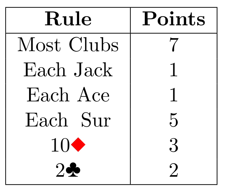
At the end of the game, each player counts their score based on the cards they have collected, using the scoring system. The scoring system is as follows: any player with at least 7 clubs receives 7 points. Each Jack and each Ace is worth 1 point. There are also two key cards: the 10 of Diamonds, which is worth 3 points, and the 2 of Clubs, which is worth 2 points.
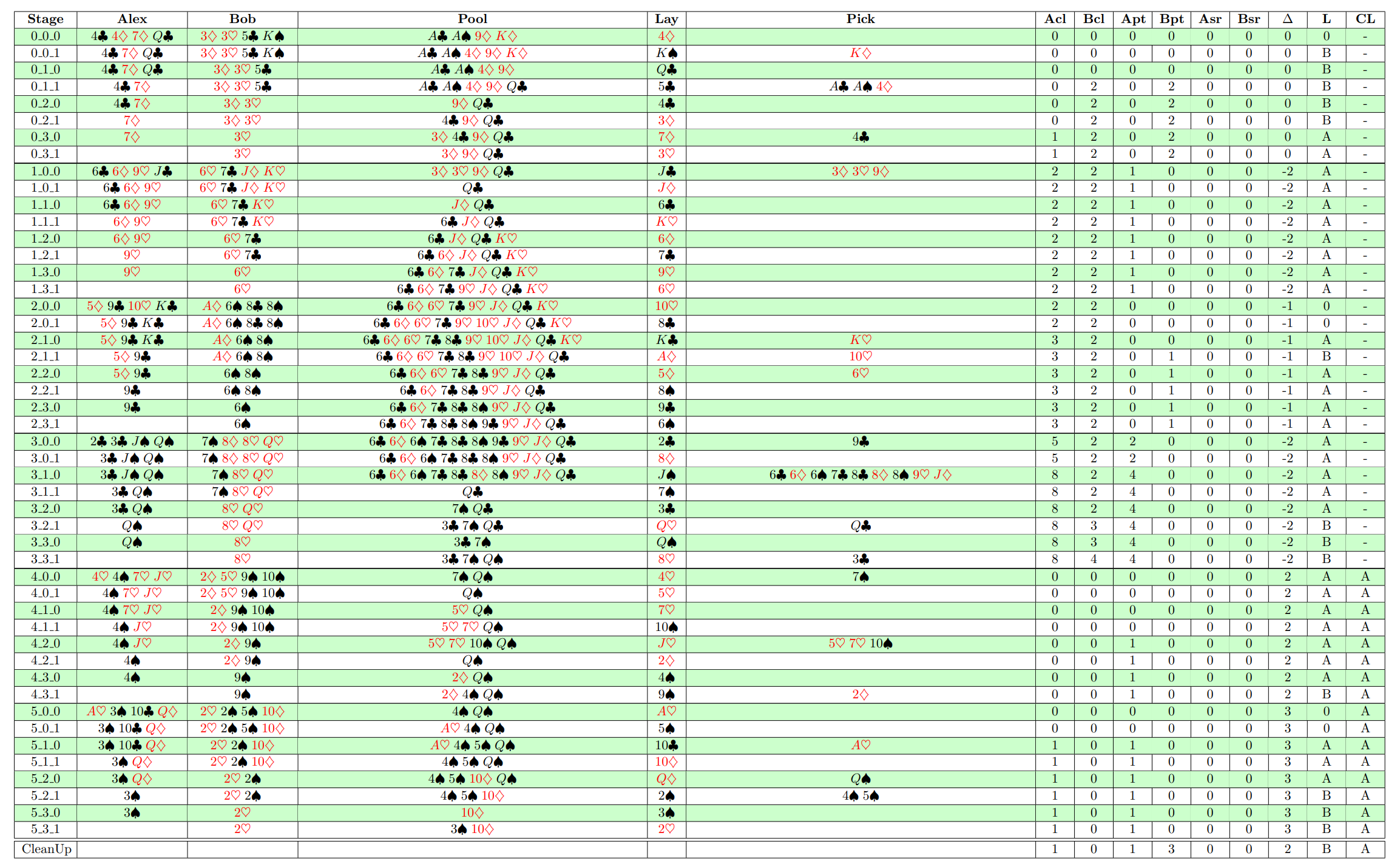
Here is an example of a full game being played. Notice the 6 rounds, and the fact that at the end of each round all the cards remaining in the pool carry over to the next round. Also, both players end each round with empty hands and are then dealt 4 new cards for the next round.
Unfolding Process
And below is a basic but key observation thatI will use to represent the full game tree, which has on average 2 to the power of 30 nodes, in a more compact way. In other words, if for two terminal nodes of the k-th round the pool carried over to the next round is the same, and the accumulated scores for Alex and Bob up to that point are also the same, then I may potentially consider the resulting root node of the next round to be identical. Notice that the score data I need to keep track of includes the number of club cards held by Alex and Bob, as well as the point difference from the point cards. I also add an extra value to the score to record whether Alex or Bob has accumulated at least 7 clubs by that terminal node of the round. In that case, I reset the number of clubs for both players to zero and set this new index to 1 or 2, depending on whether Alex or Bob was the one who collected the 7 clubs.

Based on this observation, I represent each node of the full game tree using two tensors: one is the score tensor, and the other is the game state tensor. The game state consists of the cards held by Alex and Bob, the cards in the pool, and the action history within the round. Note that at the beginning of each round, the game state resets to only reflect the card status.
Pytorch Framework
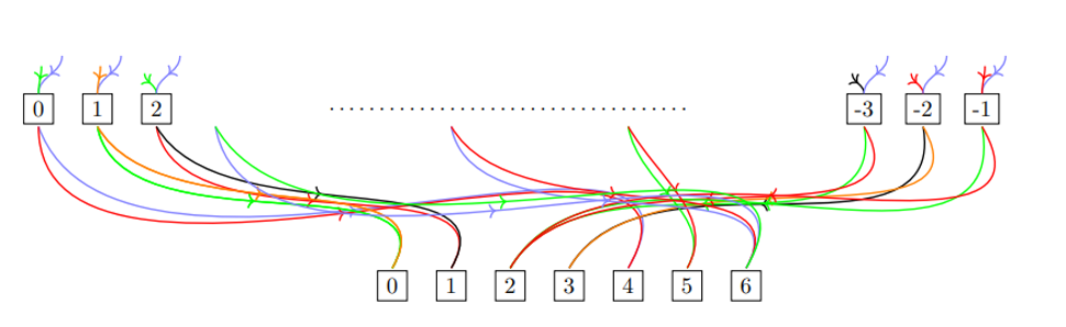
This process is explained more clearly in the figure below. I represent the inherited scores from previous rounds using colored arrows going into a node. I call the left-hand side the Game Tree and the right-hand side the Full Game Tree. Notice that the branching factors are shown by the underlying lines. For example, here the branching factor is [2, 3].
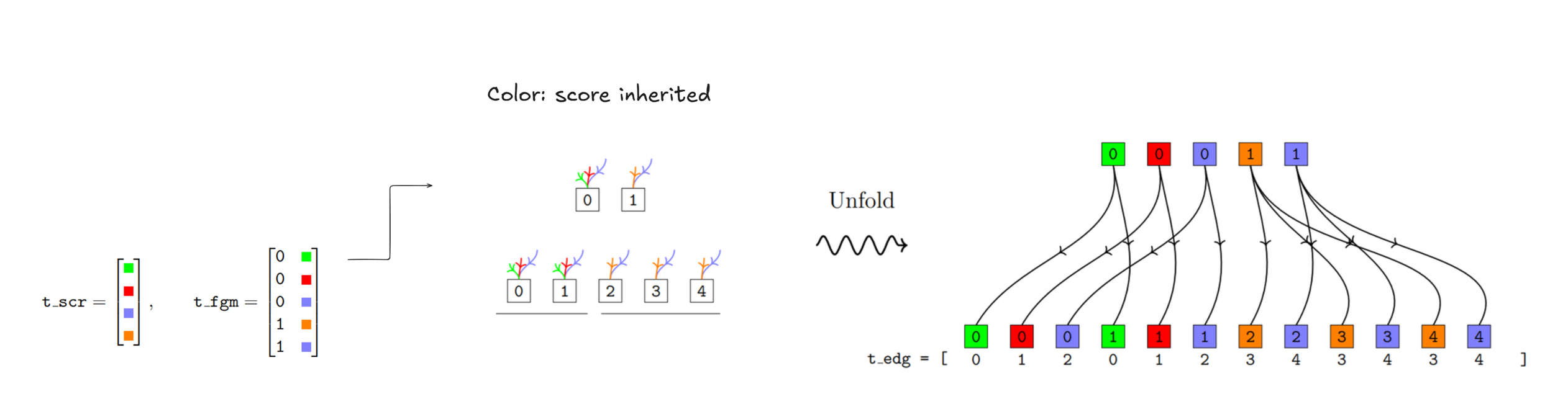
I need to explain the unfolding process—how to convert the Game Tree into the Full Game Tree. For now, let me mention the 4 main tensors used throughout. The first is the game tensor t_gme, which encodes the card states and action history within each round. The second is the score tensor t_scr, which encodes all the unique scores inherited from previous rounds. And finally, the Full Game Tree tensor, t_fgm, where a [g, s] entry means that the g-th row of the Game Tree has inherited the s-th score from t_scr. Connections between the layers of the Full Game Tree are also encoded in the t_edg tensor, as shown in the figure above.
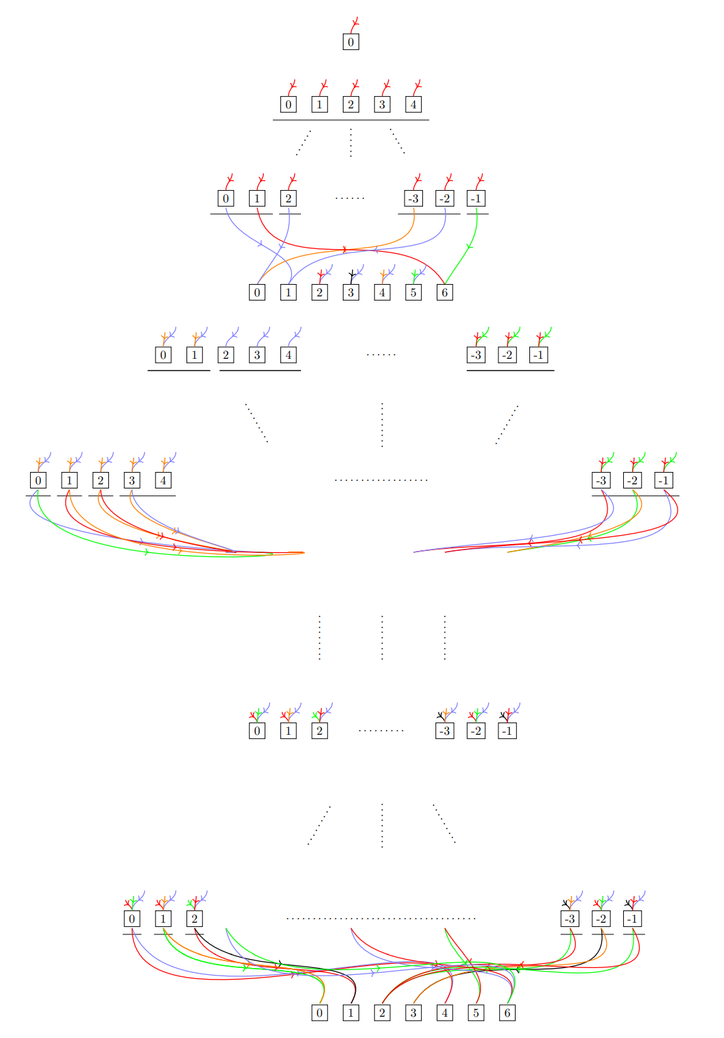
The next figure shows the game tree of height 48. Notice that in the first round, all the incoming arrows are colored red, because at the start of the game all scores are identically zero. In other words, nobody has collected any cards at that point. Throughout, I refer to this as the Game Tree (GT) and the Pasur Full Game Tree as shown above the Full Game Tree (FGT). Note that FGT is preserved through the full game tensor t_fgm and also the score tensor t_scr.
At this stage, I need to explain several things, including how PyTorch tensors are used to represent game states. I also need to explain how these tensors are updated throughout the process.
Game Tensor
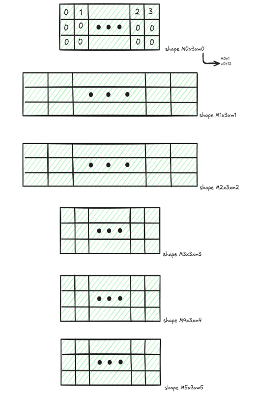
So let me explain the game state tensors. Each layer of the game tree is represented by a tensor of shape M × 3 × m. Here, M is the number of nodes in that layer, and m is the number of active cards. A card is inactive if it has not yet been played or if it has already been collected across all terminal nodes of the previous rounds.
So let’s look at a slice of a game tensor. Each slice corresponds to a node in the game tree and contains 3 rows.
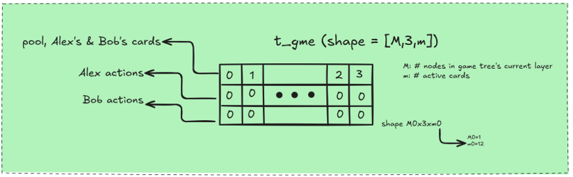
The first row encodes card ownership: 1 means Alex has the card, 2 means Bob has the card, and 3 means the pool contains the card. A value of 0 means the card has already been collected or is only active in another node of the game tree.
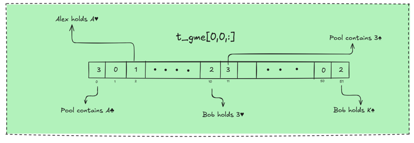
The second row encodes Alex’s action history. A value of 1 is added if a card is laid on his first turn, and 10 if it is picked on his first turn. Values of 2 and 20, 3 and 30, 4 and 40 are used similarly for the later turns.
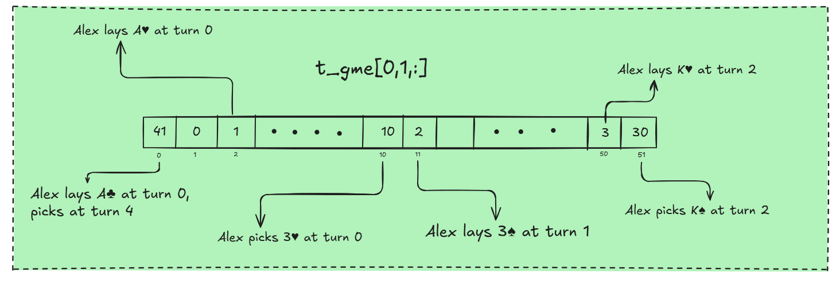
Notice that a value of 41, for example, means the card was laid on the first turn and picked on the fourth turn. Similarly, a card that is laid and picked in the same turn can be identified by a value of 2 for that turn in the second row, while the corresponding value in the first row of the game tensor is 0.
Keeping track of inactive cards results in significant memory savings, as tensor sizes are kept optimally small. I also maintain padding tensors to help consolidate different tensor shapes whenever needed.
Next, I will explain how game tensors are updated throughout the process. There are two types of updates: in-hand updates and between-hand updates.
In-Hand Updates
Let us begin with the in-hand updates. Consider the example above with two game nodes, where the inherited scores are 3 and 2. In this case, the count score tensor c_scr is given by [3,2]. Assume further that the branching factors are 2 and 3; t_brf = [2,3]. This setup corresponds to the figure on the left-hand side. Observe the count score tensor alongside the branch factor tensor. The complete game tensor for the first row of the game tree is also displayed. The right-hand side illustrates the unfolded Full Game Tree. The unfolding is constructed in the most natural way: each node of the game tree is repeated with the same label but shown in a different color, depending on the incoming colors within the tree. The next step is to identify the edge tensor, which maps each node in the second layer of the Full Game Tree to its corresponding node in the first layer.
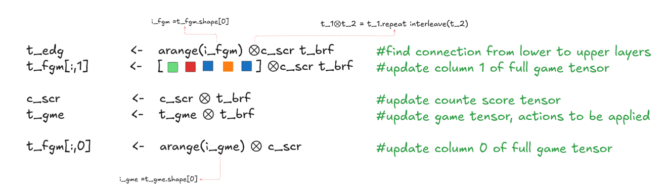
Here, the \(\otimes\) notation refers to the PyTorch repeat_interleave operation. I also use an extension of repeat_interleave, which I call repeat blocks. This operation divides the source tensor into chunks and repeats each chunk a specified number of times. Notice that only nodes with matching colors are connected.
A simple inspection shows that the edge tensor is constructed using the displayed formula via the repeat-blocks process. Block sizes are determined by the count score tensor, and the repeat tensor is given by the branching factor. The first block [0, 1, 2] is repeated twice, while the last block [3, 4] is repeated three times, since its branching factor is 3. Similarly, column 1 of the FGT is updated. Recall that this column encodes the color of each node in the FGT.
After these two updates, I proceed to update column 0 of the FGT tensor. Before doing so, the count score and branching factor are updated. Note that the actions will be applied to the game tensor at a later stage.
Between-Hand Updates
Now I explain the between-hand updates. Remember that at the end of each round, the pool and the inherited scores are the only items that matter. I discard all other information in the game tensor except for the pool formation. I then find the unique pool formations using torch.unique. Notice that there is no need to sort the output, but I do need to record the inverse mapping from the unique operation. I apply the same procedure for the running score tensor t_rus.
I find the new set of unique scores to be inherited by the nodes of the next round. At each node of the full game tree, I currently have two scores: one inherited from previous rounds, recorded in column 1 of the full game tensor, and the other being the running score accumulated during the current round. The resulting pair is encoded in the tensor shown here. We then apply a unique operation on this set of pairs, sum the corresponding scores, and apply unique again to determine the set of scores to be passed to the next round.
Finally, I establish the linkage between the two rounds for the full game tree. To do this, I first determine the pair index and then locate where that pair is mapped inside the score tensor. Similarly, the index of the game state can be found, as shown in the second-to-last line of the displayed code snippet.
The game tensor is then populated using the newly dealt cards at the root level of the next round, while the full game tensor already reflects the unfolding process for that root level.
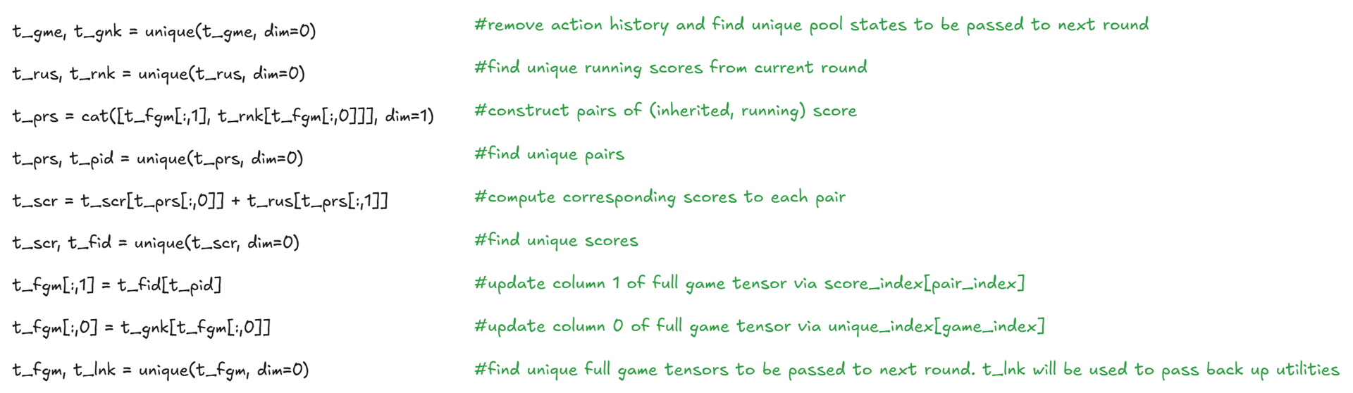
Notice that the linkage tensor is used to propagate back the utilities computed for each full game tree during the CFR algorithm. Since CFR is trained on the full game tree, I need to pass back the calculated utilities from the root level of each round to the terminal level of the preceding round.
Action Tensor
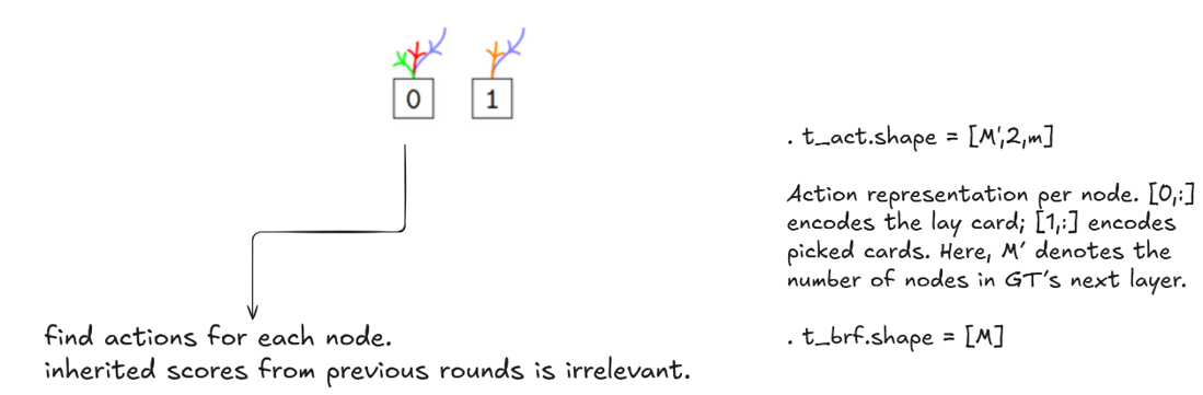
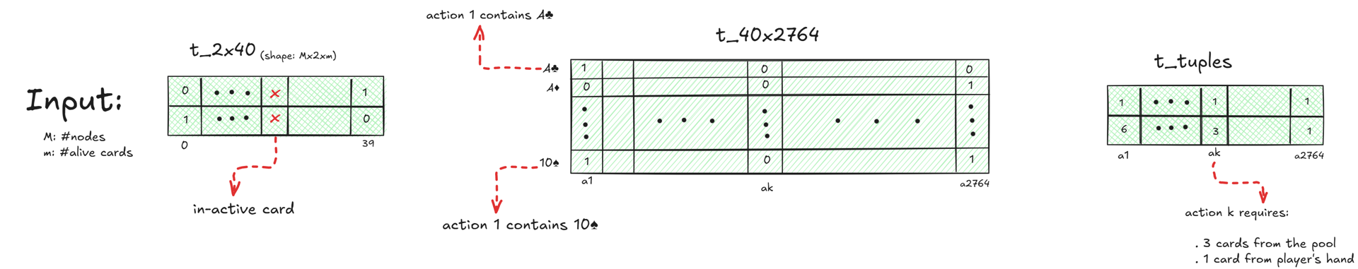
Next, I explain how the action tensor is constructed. Note that the inherited score is not important when computing actions at each game tensor node. The action tensor has shape M' × 2 × m, where M' is the number of nodes in the next layer of the game tree. The first row encodes the hand cards used in each action, and the second row encodes the pool cards used.
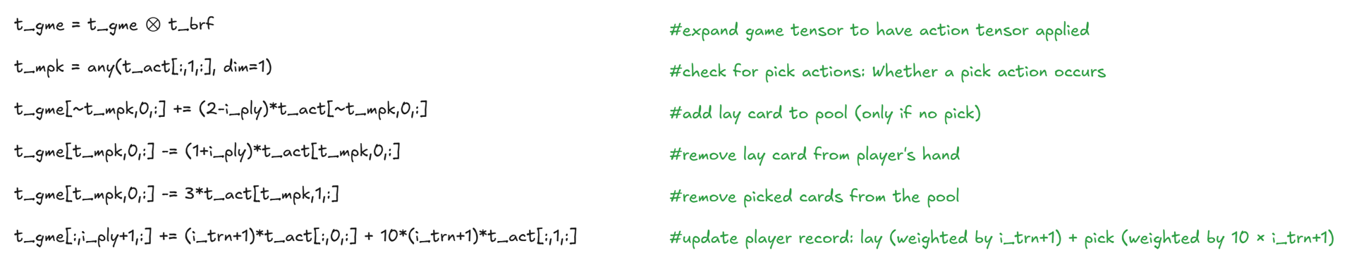
Once the action tensor t_act is obtained, the game tensor t_gme is constructed as follows. I first identify the pick actions, meaning those in which at least one card from the pool is selected. According to the rules of the game, whenever such a pick occurs, both the laid card and the selected pool cards are collected by the player. If no pick occurs, the laid card is simply added to the pool and removed from the player’s hand. t_act[*,1:2,:] is updated via the procedure explained above, that is lay (weighted by i_trn+1) plus pick (weighted by 10 x (i_trn+1)).
Actions are divided into four categories: Numeric, Jack, King, and Queen actions. For example, since numeric actions do not involve face cards, when constructing them I filter the input game tensor to mask out all cards that are not numeric. I denote the resulting tensor as t_2x40. Note that, due to the dynamic shaping discussed earlier, t_2x40 does not necessarily have shape 40; the notation is used for clarity.
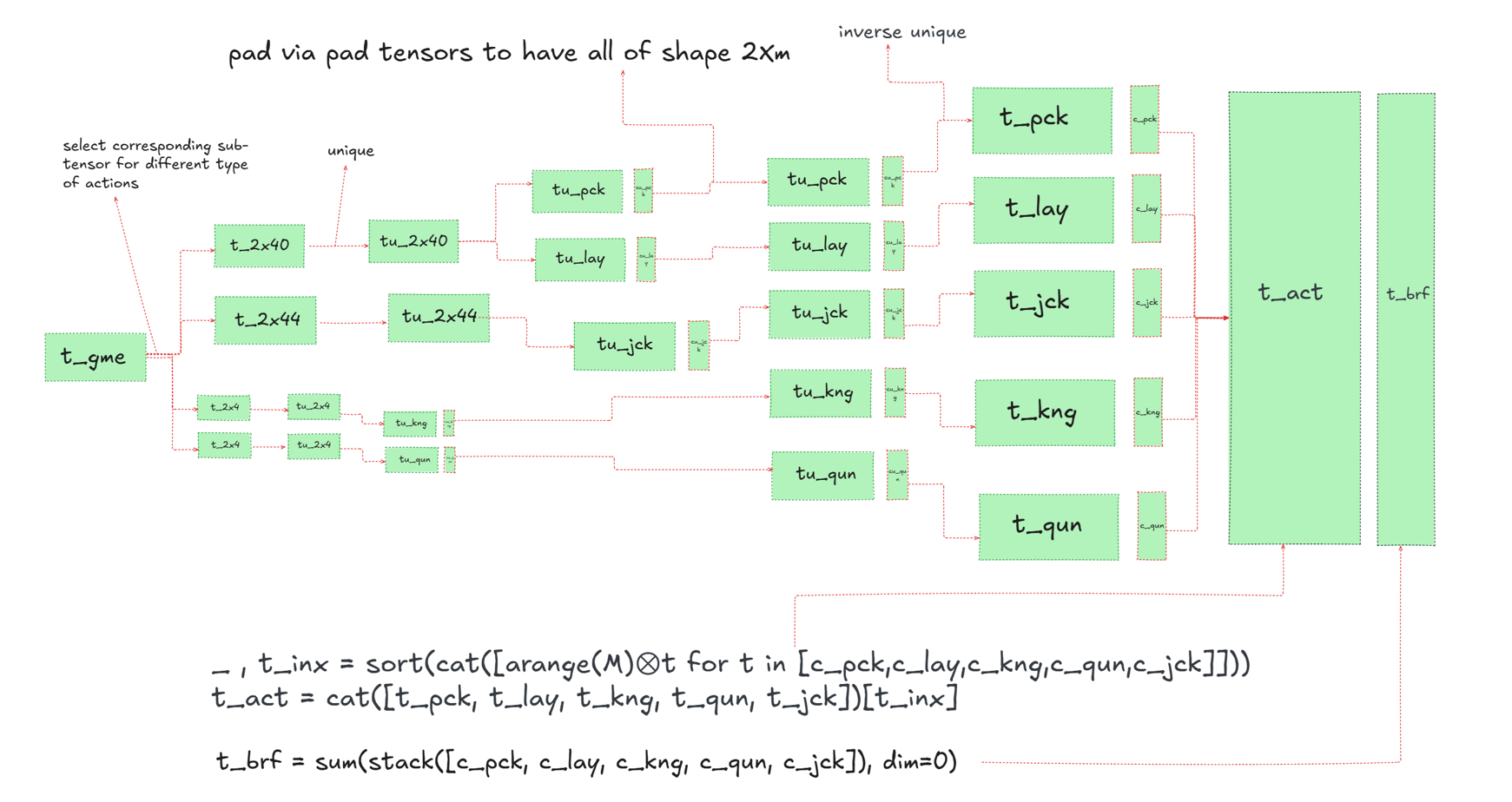
Once t_2x40 is obtained, I apply torch.unique without sorting to obtain tu_2x40, while also recording the reverse indices. For numeric actions in particular, I separate pick and lay actions and construct the resulting action tensors individually. These action tensors are denoted by tu_pck and tu_lay, along with the corresponding count tensors cu_pck and cu_lay. Similarly, I obtain tu_jck, tu_kng, tu_qun, cu_jck, cu_kng, and cu_qun.
Afterward, I apply padding to restore all tensors to the original shape of t_gme. In other words, tu_pck.shape[2] = t_gme.shape[2], and so on. Next, I reverse the unique operation. The details of this step are omitted here, but I refer you to the full paper for further explanation.
At this stage, I have the tensors t_pck, t_lay, t_jck, t_kng, t_qun, c_pck, c_lay, c_jck, c_kng, and c_qun. Finally, I concatenate the action tensors in such a way that all actions corresponding to each node of the game tree are grouped together. To achieve this, I concatenate these action tensors and then use the sorting indices obtained from the count tensors to shuffle the concatenated result, yielding t_act. The figure below summarizes this operation. The branching factor t_brf is constructed as shown.
Numeric Actions
I explain how the numeric actions are constructed. The construction of king, queen, or jack actions is not discussed here; for those details, I refer the reader to the full paper. To find the numeric actions, I first construct an auxiliary tensor t_40x2764, where each column represents a unique possible action. This can be done using a simple Subset Sum Problem application. I also create another auxiliary tensor t_tuples, where the k-th column is [1, q], with q+1 being the number of cards used in the k-th action. See figure below.
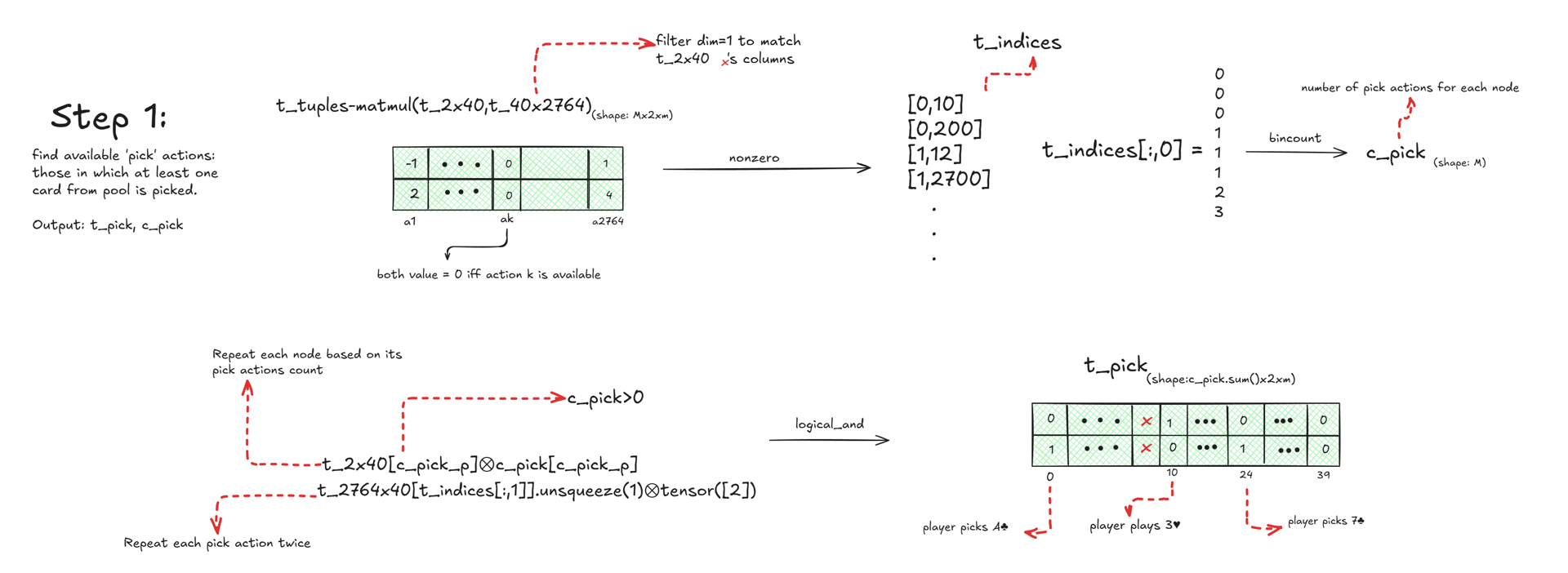
I can now easily determine whether action k is available for node i of tensor t_2x40. To do this, I compute t_tuples - matmul(t_2x40, t_40x2764). The resulting tensor has shape Mx2x2764, and its [i,:,k]-th column is 0 if and only if the k-th action is available for node i.
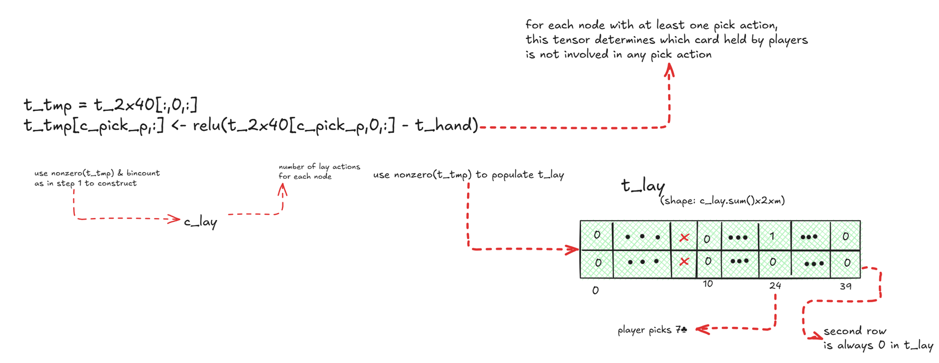
Next, I construct a tensor based on the pick action tensor t_pck, where each column corresponds to a node and each value represents the number of pick actions involving a specific card. I denote this tensor by t_hnd. The tensor t_hnd is then used to determine the available lay actions.
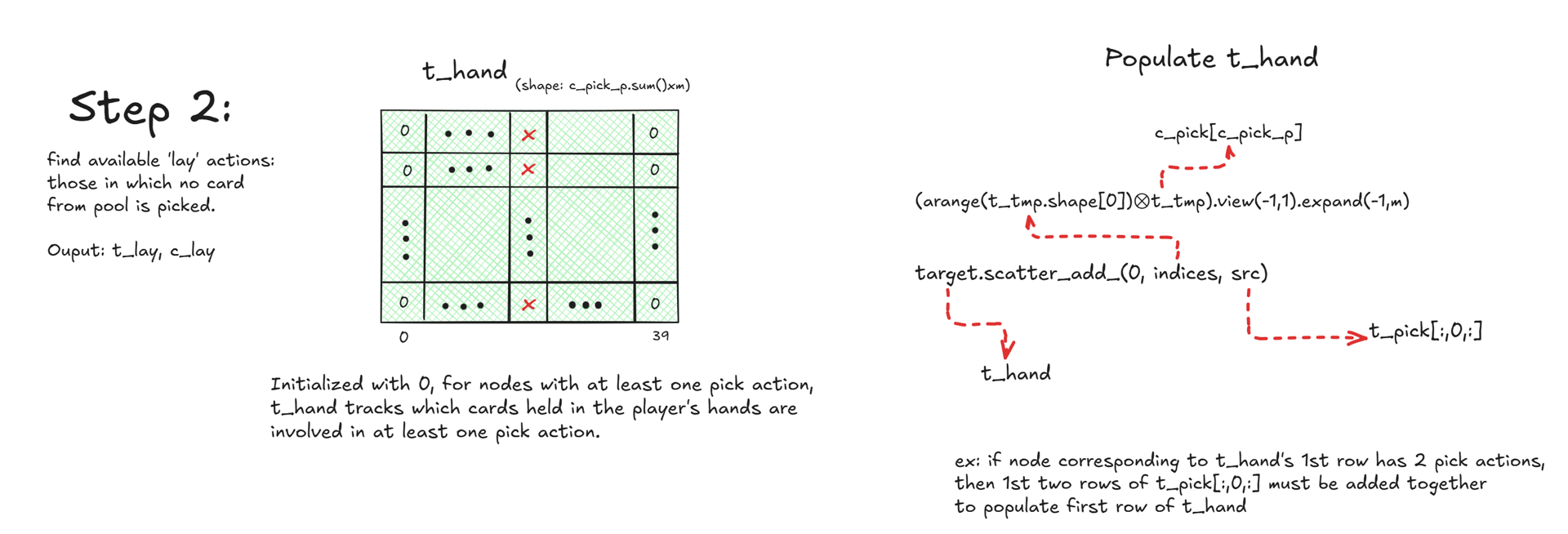
Once t_hnd is constructed, the lay cards are found using a simple torch.relu(t_2x40 - t_hnd) computation. The masking requirement is omitted here, and the details can be understood from the figure below.
Overview
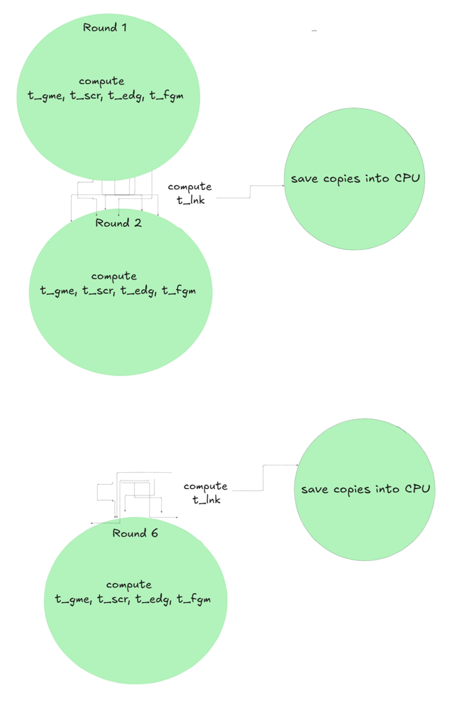
The procedure explained above describes how to generate the game tree information. Its purpose is to produce data that represents the full game tree. This data is then used to run the CFR algorithm in order to obtain the Nash Equilibrium strategies. The figure below shows the scheme of the entire process. The tensors to be saved are the game tensor t_gme, score tensor t_scr, edge tensor t_edg, and the full game tensor t_fgm. It is also necessary to preserve the linkage between the FGT nodes across rounds, which is encoded in the t_lnk tensor.
Once each round is calculated, the resulting tensors are passed to the CPU to be used in the CFR algorithm. Note that CFR is applied round by round in reverse order. Therefore, I first pass the data for round 6 to the GPU; once CFR for round 6 is complete, those tensors can be removed from the GPU, and the data for round 5 is then transferred, and so on. This approach optimizes GPU memory usage. For more details, see the sections below.
External Sampling
The current framework addresses the setting where both players are fully aware of each other’s hands. To extend this to the more realistic and challenging case where players do not have access to the opponent’s hand information, we need to incorporate sampling techniques along with approaches such as Deep CFR. For further details, see the Future Work section in the full paper. It is emphasized that implementing this extension requires substantial computational resources.
Figure below illustrates external sampling.
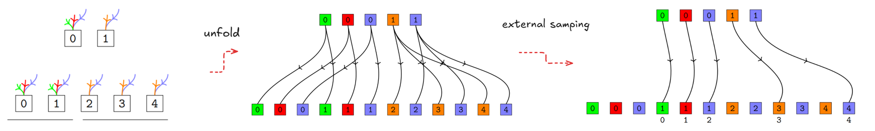
The figure below also illustrates the mechanism for external sampling. Here, c_edg counts the number of edges for each GT node. It can be obtained via c_edg = t_brf ⊗ c_scr.
CFR Implementation
Next, I explain the details regarding the implementation of the CFR algorithm. The Nash strategies are obtained round by round, starting from the last round, namely round 6. I first compute the utilities at the terminal nodes, and then derive the Nash strategies for the nodes within that round. In other words, starting from any root-level node of round 6, I determine the optimal strategies by assuming a reach probability of 1 for each root-level node. Once the utilities at the root nodes are computed, they are passed up to the previous round, with the running score from that round added to the utilities. These updated values serve as the terminal node utilities for that round, which are then used to compute the corresponding CFR strategies.
I now explain how the CFR algorithm is implemented for a single round. The procedure consists of a forward phase and a backward phase.
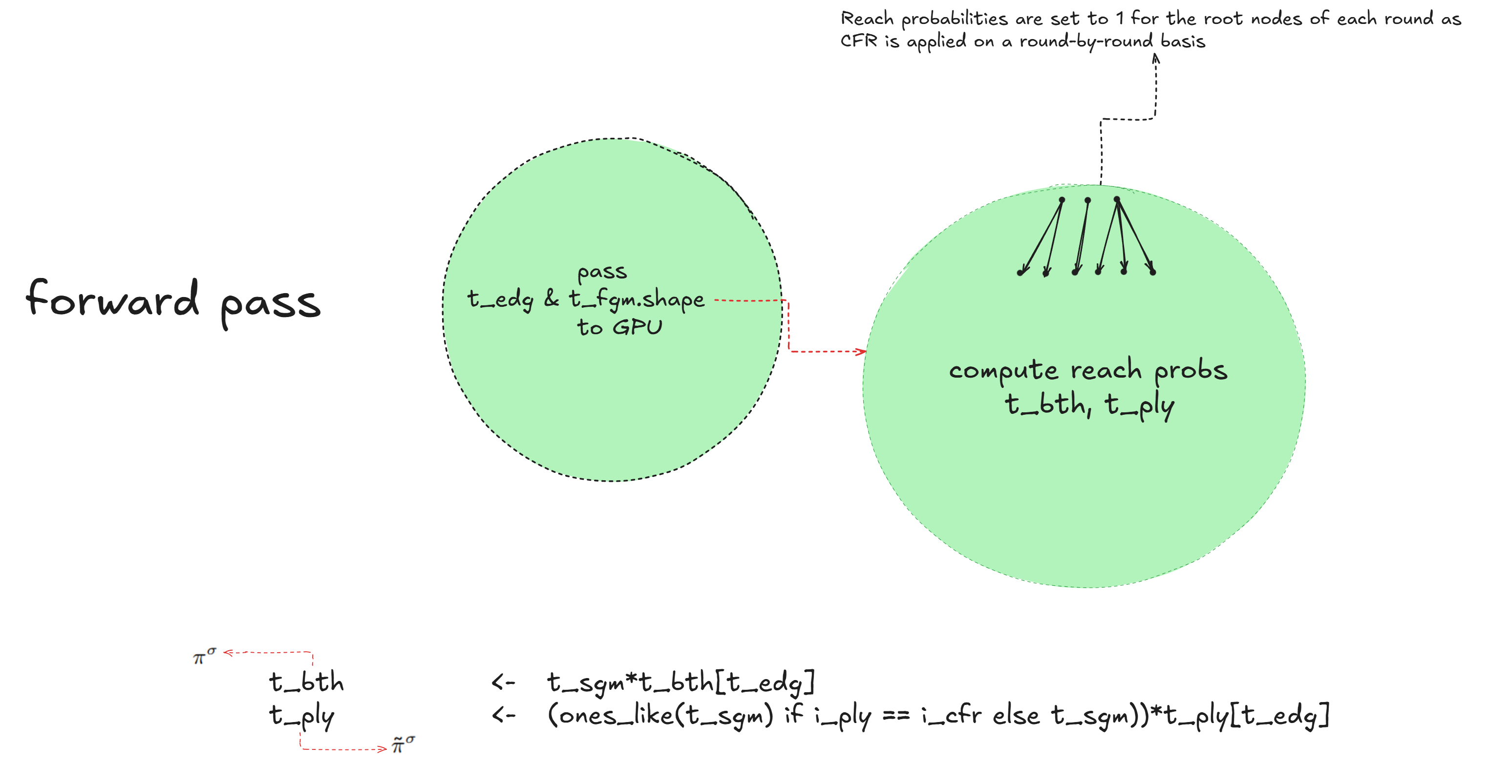
Forward Pass
In the forward phase, I compute the reach probabilities. There are two types of reach probabilities to calculate:
- The probability that both players play according to the current strategy to reach a given node, denoted by \(\pi^{\sigma}\).
- The probability that, for a given node, the player whose turn it is purposefully reaches that node, denoted by \(\tilde{\pi}^{\sigma}\).
The figure below illustrates how these probabilities are calculated.
Backward Pass
In the backward pass, I update the strategy and utility. Recall that in CFR, strategies are initialized uniformly. I begin by computing the utilities at the terminal nodes of the last round and to this end I pass t_rus, c_scr, and t_scr to the GPU to compute the utility tensor t_utl. I use the score tensor t_scr, the link tensor t_lnk, and the running score tensor t_rus corresponding to the last layer of the last round. To propagate the running score across all nodes of the FGT derived from the GT, I apply repeat_interleave(t_rus, c_scr). This step unfolds the running scores in alignment with the structure of the FGT. Once t_utl is obtained, utilities are propagated backward layer by layer to compute the action regret tensor t_reg. Note that, the reach probabilities t_ply are used in this step to properly weight regrets. I also aggregate regrets by adding t_reg to the cumulative regret tensor a_reg. Figure below illustrates an overview of this process.
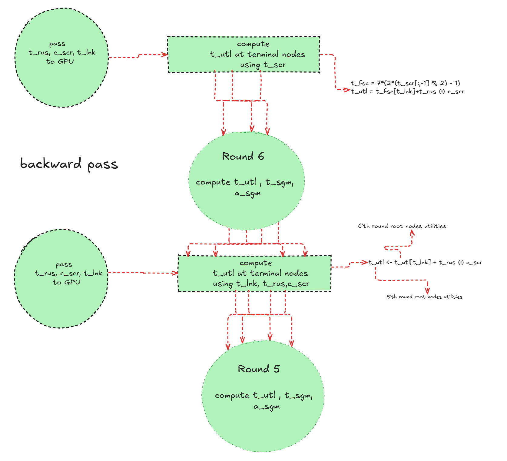
Figure below also shows how t_utl is updated. Note that the computed t_utl values for the root-level nodes are accumulated inside the a_utl tensor, which is then passed to the terminal nodes of the previous round.

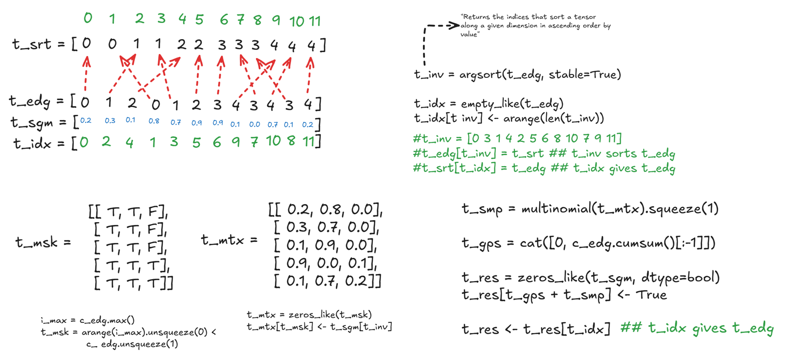
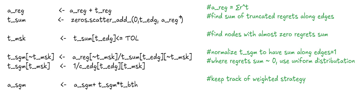
Finally, the running strategy is updated via a simple use of the scatter_add_ operator, ensuring proper accumulation across actions. Here, TOL = 1e-5 is used to handle numerical stability. For this update, the FGT layer shapes and edge tensors t_edg, which were already passed to the GPU are required. Figure below illustrates this process.
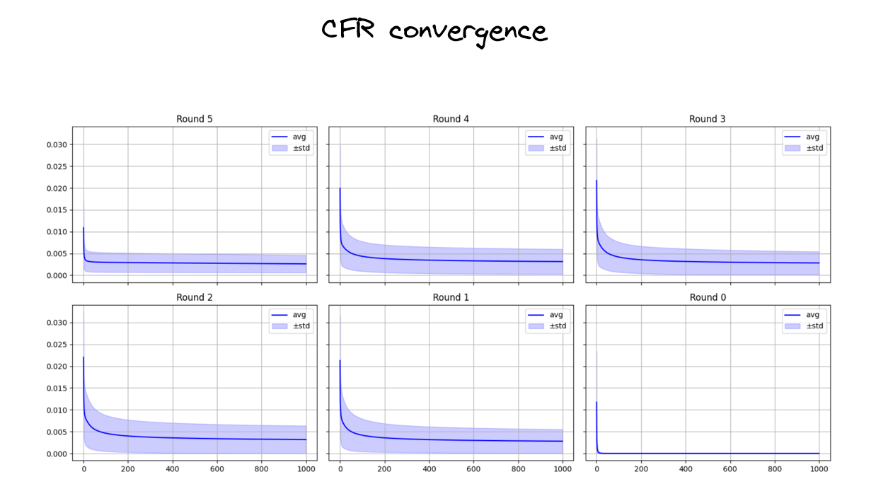
Convergence
I examine the convergence behaviour of the CFR algorithm next. For this, I run CFR (a slightly modified version compared to the one described above; see the paper for full details) over 500 randomly generated decks.
The experiments are done in two stages:
- The first run is used to obtain the Nash Equilibrium strategy.
- The second run measures the mean squared error (MSE) distance to that strategy.
For each round, I compute the mean and standard deviation of the MSE distances. The plots below show these convergence statistics separately for each round.
Model
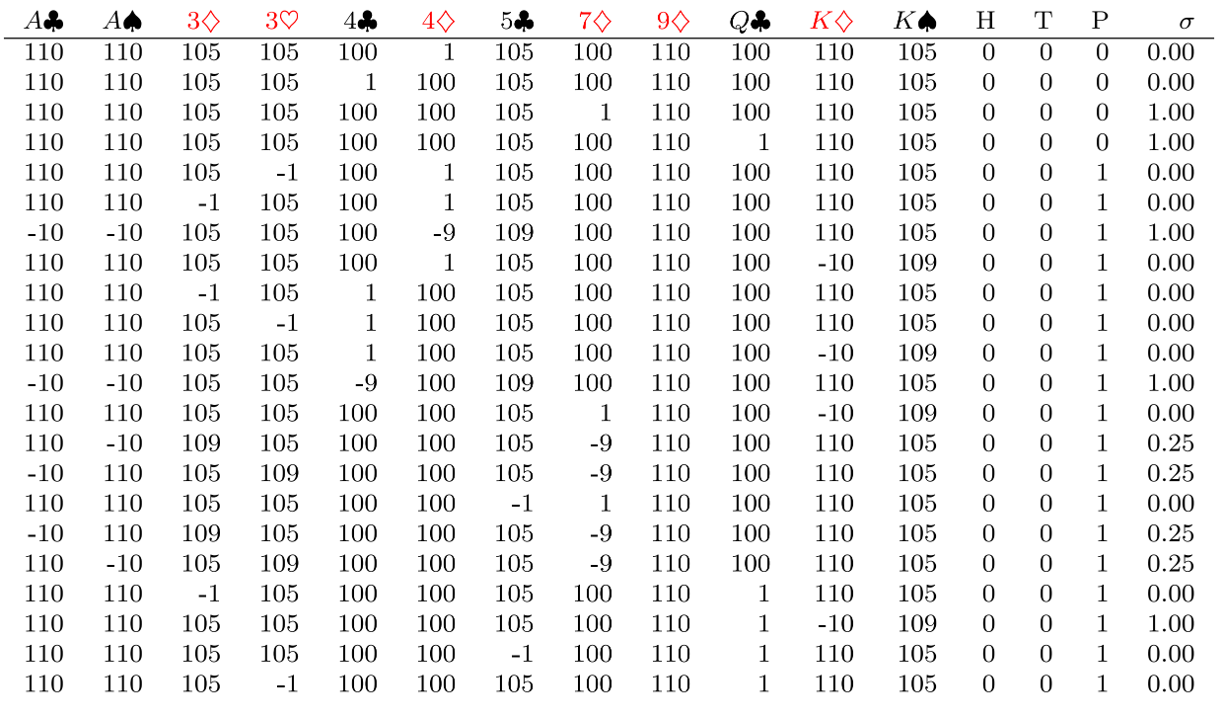
The last step is to train a tree-based model to be used as an AI agent to play the game with. To this end, I need to train a model so that it takes in the FGT node and outputs the Nash strategies obtained above. In order to represent an FGT node, I need to encode the game state, which is a 3 × 52 tensor, as well as the score inherited from the previous round.
Notice that I added three columns H, T, and P to encode the game state: whose turn it is, which round it is, and whose turn it is to play. With this encoding, I require 163 = 3×52 + 4 + 3 features and one target value, namely \(\sigma\). However, I manage to compress the game tensor data into a 52-sized tensor as explained below.
Each card within a single round has four possible states:
- Not played yet.
- Laid to the pool and not picked yet (one leg).
- Laid and picked in the same turn.
- Laid and picked at a later turn.
Based on this observation and using the difference tensor t_dff = t_gme[:,1,:]-t_gme[:,2,:], I manage to compress t_gme into t_cmp as detailed below.
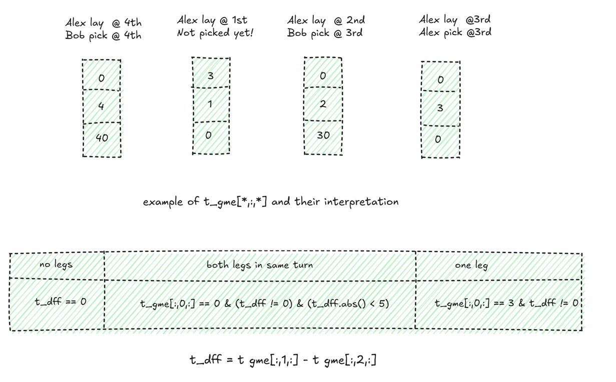
The detailed process to compute t_cmp is also illustrated below.
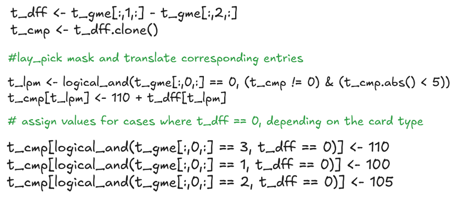
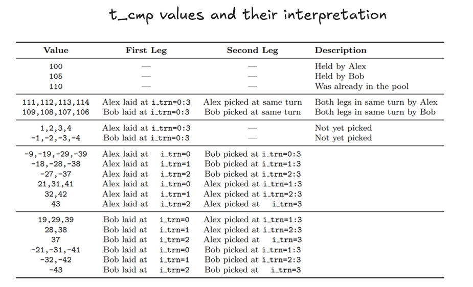
This way, the resulting compressed tensor has the possible values with the interpretation explained below.
Example
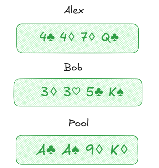
Consider the game initialization described below.
The Nash strategies obtained via CFR are displayed below. Note that score-related columns are hidden here since they are all 0 in the first round.
Experiments
I trained CFR for over 500 decks and obtained a table similar to the one above for each one. Next, I fitted an XGBoost model to predict the \(\sigma\) value. The main advantage of this approach is that it enables large-scale self-play. I use this to evaluate the performance of Nash strategies against each other as well as against a random player. The figure below displays the performance comparison.
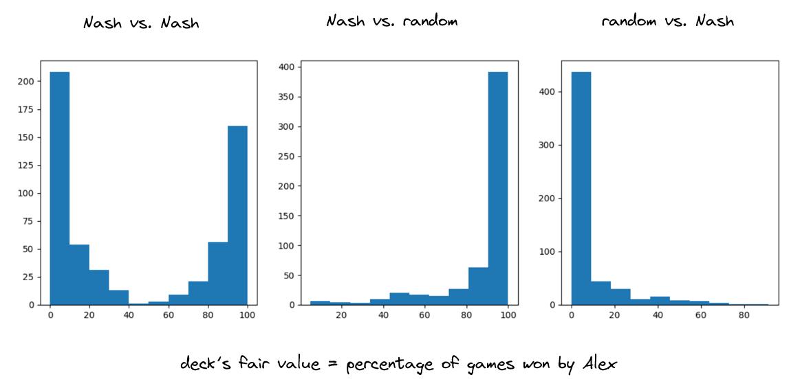
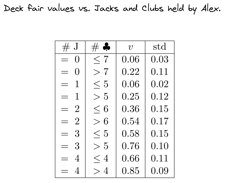
It is interesting to observe that the fair value of the deck varies significantly across different deck formations. I investigated this phenomenon and found that the variation is largely driven by the distribution of key cards. For example, players holding more clubs or jacks have a higher chance of accumulating points.
The table below reflects this observation.