Solvable Sokoban Without a Solver via Diffusion
This repository is dedicated to the paper Solvable Sokoban Without a Solver via Diffusion.
This work presents a transformer-based diffusion model for generating Sokoban puzzles. The training pipeline is adapted from the MD4 paper [1], and the dataset is DeepMind’s Boxoban [2]. The final model, along with instructions for generating new puzzles, is available here. See here for a playground of already-generated puzzles.
Determining Sokoban solvability is a PSPACE-complete challenge that demands exhaustive search to verify since even a single misplaced wall can silently render an entire puzzle unsolvable. In this work, we show that a 4.9M-parameter discrete diffusion model trained purely on tile completion, with no access to solvers, rewards, or solvability labels, achieves an unfiltered playability rate of 77.4%, with 94.5% of the remaining failures rendered solvable by removing a single wall. That a global, search-heavy property should follow from a purely local training objective is the result this work reports: by factorizing the intractable 100-cell joint distribution into a sequence of conditional steps, the model reproduces a distribution whose support consists entirely of solvable puzzles, and inherits solvability without ever being trained on it.
AI usage
The research question, model architecture, training setup, and all experimental design decisions are the author’s. Claude Code was used as an implementation and editing assistant.
Contents
Preliminary
This section is organized as follows. We first define the game of Sokoban, how a puzzle’s solvability is decided using a push-based solver, and how its difficulty is measured. We then describe the masked diffusion model: its mechanism, its evolution from the continuous-diffusion formulation, and its suitability for Sokoban puzzle generation.
Sokoban
Sokoban is a single-player puzzle created in Japan around 1980. Played on a grid-based maze with a single character and multiple boxes, the objective is to move all boxes onto designated target positions. Game mechanics are strictly restricted to pushes meaning that the player can only push one box at a time into an adjacent unoccupied space and cannot pull boxes.
Due to spatial interdependencies, Sokoban cannot be decomposed into isolated tasks. Moving a single box alters board topology and player reachability; an incorrect execution order can obstruct future paths or render previously placed boxes into deadlocks. Sequence is therefore as vital as destination. Because localized, step-by-step decision-making fails, players must formulate a holistic plan accounting for all box interactions prior to execution.
Solvability
A puzzle is solvable if some sequence of legal box pushes lands every box on a goal. We decide this with a push-based solver that branches on pushes, not on player moves. The player’s individual steps only relocate the worker without changing the puzzle, so branching on every movement would blow up the search with positions that differ solely in where the player stands. Instead we branch once per box push, and normalize the player to the region it can currently reach: every board with identical boxes and the player anywhere inside that reachable region collapses to a single search state. Branching is therefore tied to the box configuration rather than to navigation. We also prune dead cells: working backwards from each goal by pulling a box outward, any cell never reached is one no box could ever be pushed to a goal from, so pushes into it are discarded rather than branched on.
Culberson [4] proved that deciding Sokoban solvability is PSPACE-complete. PSPACE is the class of problems solvable with a polynomial amount of memory, though possibly requiring exponential time, and it contains NP. What separates Sokoban from an NP-complete puzzle such as Sudoku is that its shortest solution can be exponentially long: there is no short certificate that a checker could verify quickly, so establishing that a puzzle is solvable may require searching an enormous state space.
Difficulty
Jarušek and Pelánek [3] modeled Sokoban difficulty on the push-based state-space graph $G = (V, E)$, where each vertex $v \in V$ is a game state (box positions plus the player’s reachable area) and each directed edge $e = (u, v) \in E$ is a single valid box push. Evaluating metrics against large-scale human solving logs, they found that static, global properties of the graph fail to predict human difficulty: push-space size $\vert V \vert$ showed no significant correlation ($r = -0.11$) and shortest push-solution length $L$ was only weakly predictive ($r = 0.30$). What did predict difficulty were metrics modelling the search a human actually performs, rather than properties of the finished graph. Two stood out. A decomposition metric, measuring how far a puzzle breaks into independent sub-problems that can be solved one at a time, reached $\rho = 0.82$ under Spearman correlation. A stochastic model of a human wandering the state space, rather than walking the optimal path, reached $r = 0.76$ under Pearson correlation.
The difficulty measure used in this work is aligned with that finding. We rate a puzzle by the number of states the push solver expands before it finds a solution, which is a measure of how much search the puzzle demands rather than of how large its state space is. This is machine search rather than human search, so it is an analogue of Jarušek and Pelánek’s predictive metrics rather than one of them. It nonetheless falls on the same side of their distinction, and deliberately not on the side of $\vert V \vert$, which their logs show carries almost no signal.
Masked diffusion model
Continuous diffusion models are built on a stochastic differential equation (SDE) that gradually turns data into noise. Song et al. (2021) showed this process can be run in reverse in two ways: as a matching reverse-time SDE, or as a deterministic probability flow ODE with the same marginal distributions i.e., an ordinary differential equation that a standard solver can integrate directly. Both routes need the same missing piece: the score function, $\nabla_x \log p_t(x)$, the gradient of the log-density of the noised data at each step. The score function has no closed form; it can only be estimated by training a separate network against a score-matching objective. Every part of this, meaning the SDE, the ODE, the gradient, the density is defined over a continuous, differentiable space. None of it has a meaning for discrete data: there is no gradient of a distribution over seven tile types, and no log-density of a word.
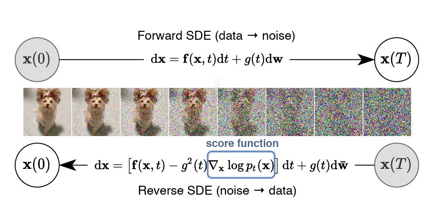
Figure 1 from Song et al. (2021), reproduced here. Top, forward SDE: the process that corrupts data $\mathbf{x}(0)$ into noise $\mathbf{x}(T)$, shown corrupting a photograph step by step. Bottom, reverse SDE: the same process run backwards, turning noise back into data. This is made possible only if the score function $\nabla_{\mathbf{x}} \log p_t(\mathbf{x})$, boxed in the equation, is known at every intermediate step.
The diffusion models that generate images work on continuous data. The forward process gradually adds Gaussian noise to a picture until nothing is left but static; the model learns to run that backwards, removing a little noise at a time. Discrete data however breaks that. A Sokoban cell is a wall, or a floor, or a box; there is no “slightly noisy wall”, and nothing sensible halfway between a wall and a box. Gaussian noise has nothing to act on.
Austin et al. (2021) built a genuinely discrete diffusion process instead, replacing the SDE with a Markov chain over categorical transition matrices where no score function required. However, the resulting training objective was still a fairly involved categorical ELBO. Shi et al. (2024), in MD4: Simplified and Generalized Masked Diffusion for Discrete Data, showed that for the masking case, specifically, this collapses to something much plainer: an ordinary cross-entropy loss, computed only at masked positions and reweighted using the timestep. This project’s training algorithm follows the MD4 formulation directly.
Masked diffusion replaces noising with hiding. Corruption means swapping a token for a special [MASK] symbol, and the schedule controls how many tokens are hidden rather than how much noise is added. Generation runs that backwards: start from a fully masked grid and progressively reveal cells, predicting what belongs in each. How many are revealed per step follows from the number of diffusion steps.
In masked diffusion models commitments are final: once a cell is unmasked it can never be selected again and the sampler only ever draws from cells still marked [MASK], so a wall placed at step 3 stays a wall for the rest of generation. Continuous diffusion has no such rule: every pixel is nudged at every one of its steps, all the way to the end, so an early bad direction can still be pulled back later.
Contribution
We train a masked diffusion model to generate Sokoban puzzles, using the formulation from the MD4 paper Shi et al., 2024. The training data is DeepMind’s Boxoban dataset. Puzzles here are $10\times10$ grids of tiles rather than sentences of words: each one flattens to 100 tokens over a vocabulary of 7 tile types (# wall, space floor, @ player, $ box, . goal, * box-on-goal, + player-on-goal), plus a [MASK] symbol the model uses but the data never contains.

Solvability emerges without supervision
Trained only to fill in masked cells, with no solver, reward, or solvability label in the loop, the model generates puzzles that are 77.4% solvable unfiltered, rising to 98.7% once failures repairable by deleting a single interior wall are counted. Here 50,000 puzzles were generated using our model and every unsolvable puzzle was checked. Counting two-wall repairs as well, only ~0.40% of everything generated is genuinely broken. Interestingly, the culprit walls were committed at a median probability of 0.45, against 0.93 for the other interior walls of the very same puzzles.
Distribution match
The tile-pattern divergence between generated puzzles and the training corpus sits on the divergence between real held-out puzzles and the same corpus, at every sample size from 250 to 50,000, where the held-out split runs out. Both series decay at the same rate, and what separates them is under 4% of the divergence itself at every size. Solvability is simply inherited from the training dataset.
Temperature trade-off
Lowering $\tau$ from 1.0 to 0.6 raises solvability by 3.8 points but inflates average wall count from 68.9 to 73.2 in the temperature sweep, against a corpus average of 68.6, while cutting median solver effort by 36%. The default $\tau = 1.0$ is the setting at which generated puzzles match real wall density.
Method and design choices
This section lays out the design of the model and the reasoning behind each choice. We first motivate why a diffusion model, rather than an autoregressive one, suits Sokoban generation. We then describe the training objective and work through the three choices that shape it: the loss weighting that keeps every noise level contributing usefully, the number of diffusion steps, and the noise schedule. Each is presented not just as a setting but with the argument for why it takes the value it does.
Model choice
The non-local interdependence between different parts of the puzzle is what makes it difficult, so an autoregressive generator, which commits to everything in one fixed order, isn’t a good fit for this kind of game. Diffusion does not work that way. It fills in cells in whatever order the reveal process happens to land on, and each new cell is conditioned on every cell already decided so far, wherever in the grid it sits, not on a fixed prefix that always runs in the same direction. The model might settle a goal in one corner, a wall on the opposite side, and only later the corridor connecting them, rather than reading the grid off in one fixed pass. Because a puzzle’s actual difficulty comes from exactly this kind of non-local interaction meaning a decision in one part of the grid constraining what will work somewhere else entirely, a generator that isn’t locked into a single fixed order is a better structural match for the problem than one that is.
Architecture
The generator $f_\theta$ is a bidirectional Transformer encoder ($\approx$ 4.9M parameters): $d=256$, $6$ layers, $8$ heads, feed-forward width $1024$, dropout $0.1$. Encoder only is used because the task is fill-in-the-blanks over a grid, not left-to-right generation.
It maps a masked grid $x_t\in\lbrace 0,\dots,7\rbrace ^{100}$ and timestep $t$ to per-cell logits over the $7$ real tiles, $f_\theta(x_t,t)\in\mathbb{R}^{100\times 7}$ ([MASK] is an input token only, never predicted).
First, we explain the cell embedding: Cell $i$, at grid position $(r_i,c_i)$, is embedded as
\[h_i^{(0)} = E_{\text{tok}}(x_{t,i}) + E_{\text{row}}(r_i) + E_{\text{col}}(c_i) + \tau(t)\] \[\tau(t)=\mathrm{MLP}\big(\mathrm{sinusoid}(t)\big)\in\mathbb{R}^{d}\]Here $E_{\text{tok}}, E_{\text{row}}$, and $E_{\text{col}}$ each maps an integer index to a learned $d$-vector. Separate row/column embeddings give attention the 2-D grid geometry directly rather than through a flat 1-D index. Moreover,
\[\mathrm{sinusoid}(t) = \big[\sin(t\omega_0),\cos(t\omega_0),\ \sin(t\omega_1),\cos(t\omega_1),\ \dots\big]\] \[\omega_k = 10000^{-2k/d}\]Note that the timestep term $\tau(t)$ is added identically to every cell. The embeddings then feed a standard stack of 6 standard pre-norm Transformer blocks (multi-head attention + FFN with residual connections), and a final linear layer projects each cell to logits over the 7 tiles.
Training
At timestep $t$ each cell is independently replaced by [MASK] with probability $1-\alpha_t$, on a linear schedule $\alpha_t = 1 - t/T$ with $T = 100$. At $t=0$ the grid is intact; at $t=T$ it is entirely mask. A training data point then consists of a sampled puzzle from the training data, a sampled $t \in {1,\dots,T}$, and a masked version of the chosen puzzle via the scheduler. The model is then trained to recover the original tokens at the masked positions, where the loss is the cross-entropy weighted by
The loss function is therefore calculated as below.
\[\mathcal{L}(\theta) = \mathbb{E}_{x_0, t, m} \Big[ w(t) \cdot \frac{1}{\lvert M \rvert} \sum_{i \in M} -\log p_\theta \big( x_0^{(i)} \mid x_t, t \big) \Big]\]Here $m$ is the mask draw, with each position hidden independently with probability $1-\alpha_t$, and $M = \lbrace i : m_i = 1 \rbrace$ is the set of positions it hides, where $t \sim \mathrm{Uniform}\lbrace 1,\dots,T\rbrace$. We now explain the three remaining choices: the weight cap, the number of diffusion steps, and the schedule.
Weights. At timestep $t$ only $100 \cdot t/T$ cells are masked in expectation, so at $t=1$ the model is graded on roughly one cell and at $t=T$ on all hundred. Without reweighting, a step that hides a single cell contributes as much to the gradient as one that hides the entire grid. The $1/(1-\alpha_t)$ factor which falls out of the masked-diffusion ELBO restores the per-sequence scale. Moreover, since $T/t \to \infty$ as $t\to 0$, with uncapped $w(t)$ a single near-complete grid would carry $T\times$ the gradient weight of a fully-masked one, and the gradient becomes dominated by a handful of nearly finished examples. Small $t$ is the near-complete regime, in which a grid has only a handful of cells left to fill. These are the cells that are critical for solvability. $w_{\max}$ therefore sets how much the model learns about the phase that determines the global property it is never trained on.
Number of diffusion steps. Notice that $T=L$ is the unique value where, first, exactly one cell is revealed per step and, second, no trained timestep is left unused by the sampler. Every reveal-step must unmask at least one new cell, so sampling always runs $\min(T, L)$ reveal steps. Choosing $T < L$ forces the sampler to reveal more than one cell per step; choosing $T > L$ leaves the sampler visiting only $L$ of the $T$ trained timesteps, so most are never used at inference.
Scheduler. As mentioned above, since the loss is computed only at masked positions, a timestep with few masked tokens carries little information per gradient step, and the uncapped weight $w^\star(t) \equiv 1/(1-\alpha_t)$ compensates by amplifying it. The schedule decides how sharply this amplification grows as $t$ approaches its minimum. Under the linear and cosine schedules, near $t=0$ the masked fraction behaves as
\[1-\alpha_t^{\text{linear}} = \frac{t}{T}, \qquad 1-\alpha_t^{\text{cosine}} \approx \frac{\pi^2 t^2}{8T^2}\]i.e., a linear vs. a quadratic falloff, so the uncapped weights grow as
\[w^\star_{\text{linear}}(t) = \frac{T}{t}, \qquad w^\star_{\text{cosine}}(t) \approx \frac{8T^2}{\pi^2 t^2}\]The cosine weight therefore diverges quadratically in $1/t$ rather than linearly, reaching $w^\star(1) \approx 8106$ against linear’s $w^\star(1) = T = 100$ which is a bounded ceiling equal to the sequence length itself.
Finally, the snippet below summarizes the training algorithm, following [1].
Algorithm 1 Training Step
Require: Batch of puzzles $\lbrace x_0^{(b)}\rbrace_{b=1}^{B}$, model $f_\theta$
- Sample $t^{(b)} \sim \mathrm{Uniform}{1, \dots, T}$ for each $b$
- Compute $\alpha_t = 1 - t/T$
- Sample masks: $m_i \sim \mathrm{Bernoulli}(1 - \alpha_t)$ for each position
- Create $x_t$: replace $x_0^{(i)}$ with $[\mathrm{MASK}]$ where $m_i = 1$
- Forward pass: $\text{logits} = f_\theta(x_t, t)$
- Average cross-entropy over the masked positions
- Apply weight $w(t) = \min(1/(1 - \alpha_t),\, w_{\max})$
- Backpropagate and update $\theta$
In Algorithm 1, training is shown for a single puzzle; the implementation vectorizes over a batch of $B$.
Loss and solvability
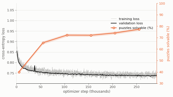
The model was trained for 1,000 epochs over the 450,000-puzzle corpus, 292,000 optimizer steps at batch size 1,536, using AdamW (learning rate $2.45\times10^{-4}$, weight decay 0.01, 125 warmup steps, cosine decay, gradient clipping at 1.0) in fp16 mixed precision on a single RTX 5070 Ti. Validation loss is measured every 1,000 steps on Boxoban’s held-out split, and solvability every 50,000 steps by generating 5,000 fresh puzzles from that checkpoint and running the push solver on each.
The plot below shows all three. Loss converges early and then stays flat; solvability keeps climbing to the end of the run. The training objective is a per-cell reconstruction loss, while solvability is a global property it never sees, so the two are free to decouple. It is emphasized that a run halted when the loss flattened would have given up roughly 25 points of solvability. Train and validation loss also track each other throughout, so the long run is not overfitting.
Distribution match
To assess whether generated puzzles capture the structural style of the Boxoban corpus beyond mere solvability, we evaluate the Jensen-Shannon Divergence, defined as
\[\mathrm{JSD}(P \parallel Q) = \frac{1}{2}\mathrm{KL}(P \parallel M) + \frac{1}{2}\mathrm{KL}(Q \parallel M)\]where $M = \frac{1}{2}(P + Q)$, between the empirical $3 \times 3$ sliding-window tile distributions of generated samples ($Q$) and the 450,000-puzzle training reference ($P$). Extracting 64 local $3 \times 3$ windows per $10 \times 10$ grid captures critical structural features such as corridors, corners, and dead ends. We choose $\mathrm{JSD}$ over raw Kullback-Leibler divergence because it is symmetric, bounded in $[0, 1]$, and naturally handles unobserved patterns without requiring arbitrary additive smoothing. Finally, because sample size strongly affects support coverage and raw scores, every generated $\mathrm{JSD}$ score is calibrated directly against a baseline of real held-out puzzles evaluated at the identical sample size.
The plot below compares generated puzzles against real ones on the same measurement: both series show how far a sample of puzzles diverges from the 450,000-puzzle training corpus in its distribution of local $3\times3$ tile patterns, plotted against how many puzzles went into the sample. The validation set is Boxoban’s held-out split, which comes with DeepMind’s dataset and consists of 50,000 real puzzles that were never shown to the model.
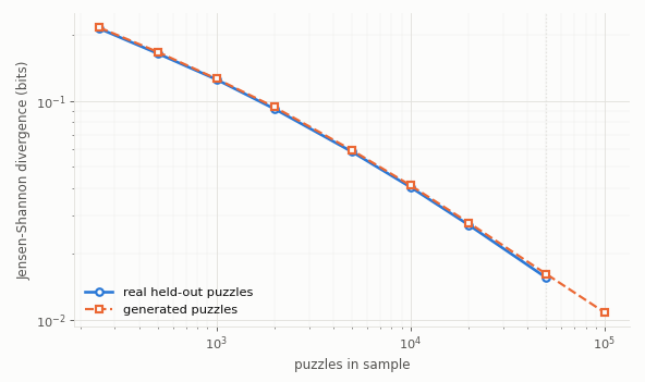
Tile-pattern JSD against the 450,000-puzzle training corpus, plotted against sample size, for generated puzzles and for real held-out puzzles measured identically. Both series decay as K−0.59: the divergence a small sample shows is dominated by how few 3×3 patterns it can cover, not by the source it was drawn from. The held-out curve is therefore the floor, and the generated curve sits on it.
Inference and evaluation
This section reports the evaluation results for the trained model: solvability, one-wall repairability, memorization, and the effect of sampling temperature. We begin with sample puzzles, rated for difficulty by the push-based search described earlier.
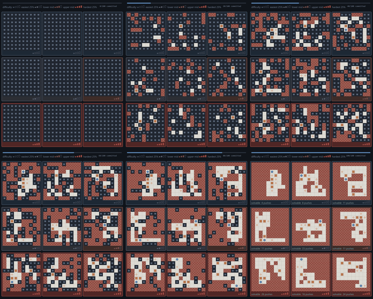
Nine puzzles generated from a fully masked grid: 100 steps, one cell committed per step in uniformly random order, never revised. Verdicts and push counts appear once every cell is committed; the bars rate each puzzle against the training corpus's difficulty quartiles.
Below are the solutions to those puzzles.
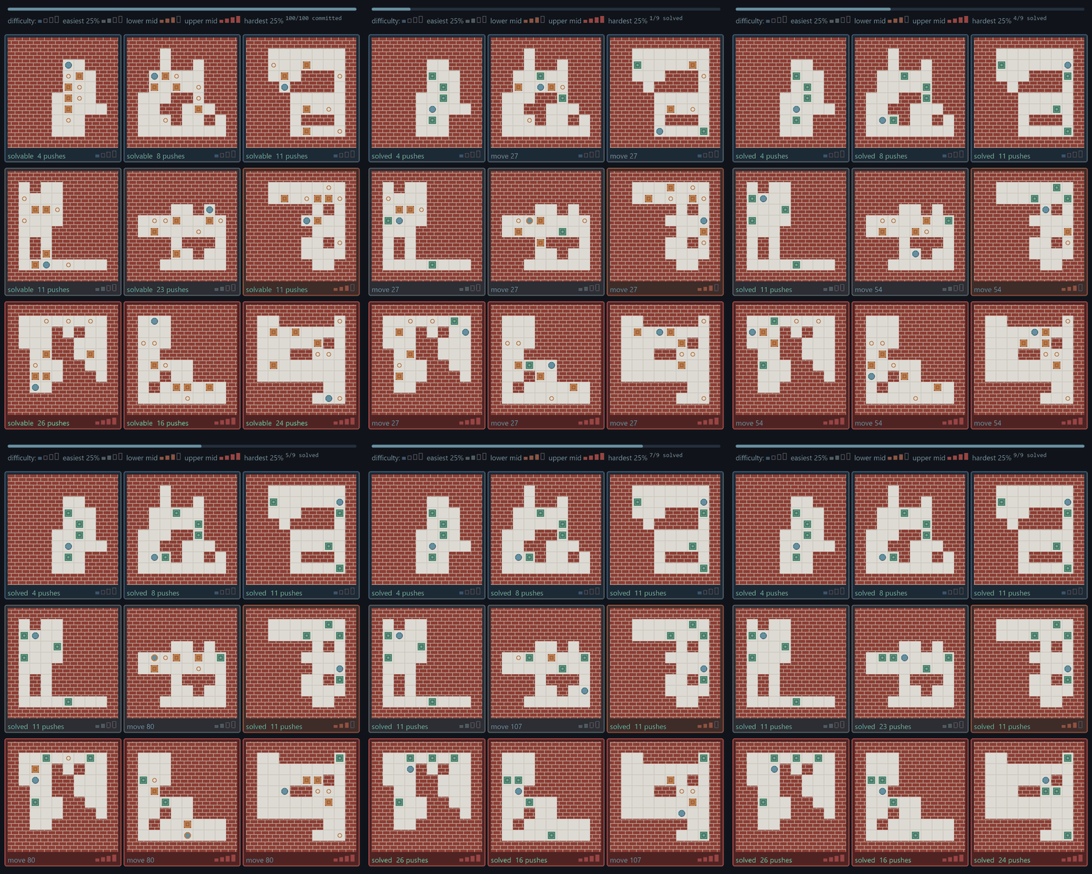
The same nine puzzles, played back under solutions found by the push-based solver.
Sampling algorithm
The generation process reverses corruption by starting with a 100-cell [MASK] grid and unmasking one cell at a time across 100 steps. At each step, the model predicts probability distributions over all seven tile types across the entire grid simultaneously. A candidate tile is sampled from each distribution—rather than selected via argmax—and exactly one uncommitted cell is chosen uniformly at random to be fixed. Discarding the remaining predictions and recomputing them from scratch on each step ensures the model chooses what tile to place while a uniform sampler determines which cell comes next. By conditioning each step on one additional finalized neighbor, the system bypasses having to model the full 100-cell joint distribution directly. In other words, the following holds
\[P(c_1, \dots, c_{100}) = \mathbb{E}_{\sigma}\left[\prod_{k=1}^{100} P\big(c_{\sigma(k)} \mid c_{\sigma(1)}, \dots, c_{\sigma(k-1)}\big)\right]\]where $\sigma$ is the random order in which cells happen to be revealed. Because training masks an arbitrary subset rather than a prefix, the model learns $p_\theta(c_i \mid c_S)$ for conditioning sets $S$ of every size and shape, which is precisely what allows any reveal order to be used at sampling time.
Selecting cells uniformly also avoids the pitfalls of confidence-based ordering: because walls are the easy, high-confidence majority class, committing high-confidence cells first biases subsequent predictions toward even more walls, inflating the average wall count in that comparison from 69.5, which matches the corpus average of 68.6, up to 81.5. The snippet below provides the inference algorithm.
Algorithm 2 Sampling
Require: Trained model $f_\theta$, $T = 100$ steps, temperature $\tau = 1.0$
- Initialize $x \leftarrow [\mathrm{MASK}]^{100}$
- for $\text{step} = 0, \dots, T-1$ do
- Compute $t = T - \text{step}$
- Forward pass: $p = \mathrm{softmax}\big(f_\theta(x, t) / \tau\big)$ for every cell
- Draw a candidate tile for every cell: $\hat{x}_i \sim \mathrm{Categorical}(p_i)$
- Collect the still-masked cells $M = \lbrace i : x_i = [\mathrm{MASK}] \rbrace$
- Decide how many to reveal: $n = \max\big(\lceil \lvert M \rvert / (T - \text{step}) \rceil, 1\big)$, which is $1$ here
- Choose which cells to reveal: pick $n$ of the masked cells in $M$ at random, all equally likely
- Commit the values sampled in line 5 at those cells (never revised afterwards)
- return $x$
One-wall fixes
When a generated puzzle is unsolvable, the failure is usually shallow rather than structural: 94.5% of unsolvable puzzles become solvable by deleting a single interior wall, which lifts effective solvability from 77.4% to 98.7%. Each puzzle below displays the probability the model assigned that wall at the moment it committed it during generation. These probabilities have a median of 0.45, against 0.93 for the other interior walls of the very same puzzles.
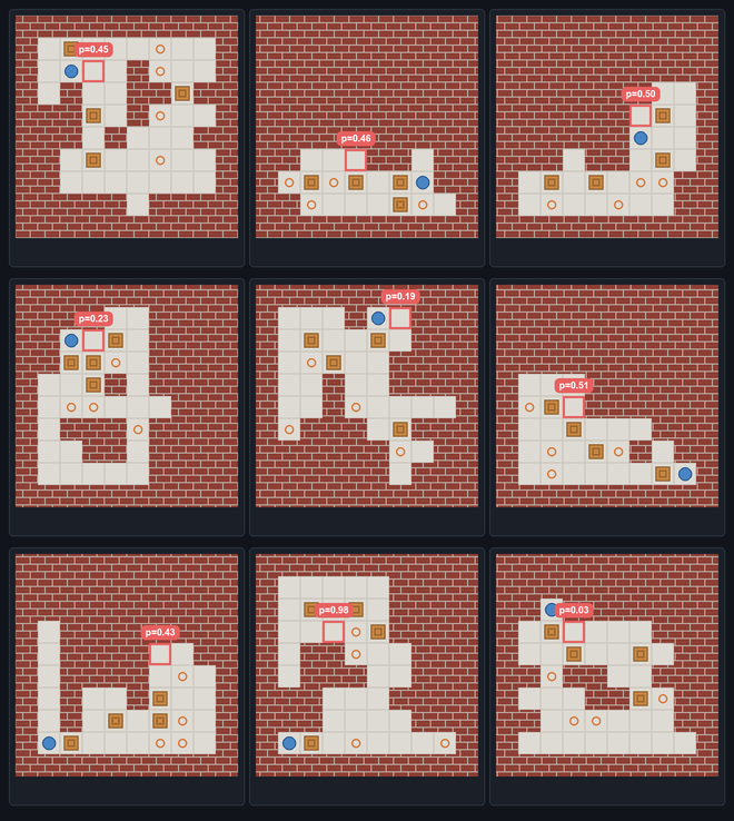
Nine unsolvable puzzles, each repaired by deleting one interior wall. The red outline marks the removed cell and the chip gives the probability the model assigned it when it was committed during generation. Measured on 11,288 unsolvable puzzles from a 50,000-sample run.
Memorization
A generator that reproduced its training data would score well on every metric above while being worthless. For each generated puzzle we measure the Hamming distance to its nearest neighbour among the 450,000 training puzzles. This is equal to the number of the 100 cells on which the two grids differ, so 0 is an exact reproduction.
The player’s position is canonicalised away before comparing. The worker moves freely within its reachable region, and the push solver collapses those positions into a single state for exactly that reason, so two grids differing only in where the worker stands are the same puzzle. Counting that as a difference would undercount duplicates.
On its own, a distance of say 12 means little: every Boxoban puzzle shares the same wall border and similar density, so unrelated puzzles already might agree on most cells. We use the 50,000 held-out puzzles as the reference. They come from the same distribution but were never shown to the model, so they cannot have been memorised. We observe that they produce the same curve once compared against the training corpus.
Over 50,000 generated puzzles and 50,000 held-out puzzles, the two distributions are near-identical: median distance 12 for both, mean 11.43 against 11.33. Exact reproductions are rarer in the generated set than in the real one, 5 against 19, as is close agreement, 5.6% within 5 cells against 7.5%. The model is therefore not copying; if anything it lands slightly further from the training corpus than genuine puzzles do.
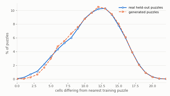
Nearest-neighbour Hamming distance to the training corpus, player position canonicalised away. Blue: for each of 50,000 held-out puzzles, the distance to its nearest neighbour among the 450,000 training puzzles. Orange: the same measurement for 50,000 generated puzzles. The blue series is the reference: it is what a generator that memorised nothing would score. Mass piled up near zero in the orange series would be memorisation; there is none.
Sampling temperature
Temperature $\tau$ rescales the logits before each cell is drawn. Lowering it sharpens the distribution toward the model’s top choice; raising it flattens it. The figure below describes the impact of temperature on wall count and solvability.
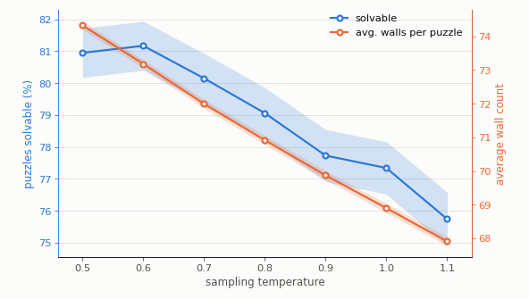
Solvability and average wall count against sampling temperature, 10,000 samples per setting on the T = 100 checkpoint. Shaded bands are 95% confidence intervals. The training corpus averages 68.6 walls per puzzle; sampling at τ = 1.0 matches it, and every lower setting exceeds it.
Citation
If you use this work, please cite it as:
@misc{baghal2026solvablesokobansolverdiffusion,
      title={Solvable Sokoban Without a Solver via Diffusion},
      author={Sina Baghal},
      year={2026},
      eprint={2608.15958},
      archivePrefix={arXiv},
      primaryClass={cs.AI},
      url={https://arxiv.org/abs/2608.15958},
}
References
[1] Jiaxin Shi et al. “Simplified and Generalized Masked Diffusion for Discrete Data.” Advances in Neural Information Processing Systems (NeurIPS), 2024. arXiv:2406.04329.
[2] Arthur Guez et al. “An Investigation of Model-Free Planning.” Proceedings of the 36th International Conference on Machine Learning (ICML), PMLR 97, 2019. arXiv:1901.03559. Dataset: https://github.com/deepmind/boxoban-levels
[3] Petr Jarušek and Radek Pelánek. “Difficulty Rating of Sokoban Puzzle.” Frontiers in Artificial Intelligence and Applications, Vol. 222, pp. 140–150, 2010. DOI: 10.3233/978-1-60750-675-1-140.
[4] Joseph Culberson. “Sokoban is PSPACE-complete.” Technical Report TR97-02, Department of Computing Science, University of Alberta, 1997.