
Generative Modeling of Heston Volatility Surfaces Using Variational Autoencoders
In this project, I focus on training a Variational Autoencoder (VAE), a generative model, to produce Heston volatility surfaces. The Heston model is a widely used stochastic volatility option pricing model. Once trained, this VAE can generate new volatility surfaces, which could be useful for various financial applications such as risk management, pricing exotic derivatives, etc. This project emphasizes the advantage of generative AI in advancing financial modeling. You can find the code for this project here.
Table of Contents
Variational Autoencoders
This section provides a brief overview of variational autoencoders (VAEs). For a deeper understanding, refer to 1. Video lectures (20 & 21) 2 are also an excellent resource for learning the core concepts of VAEs.
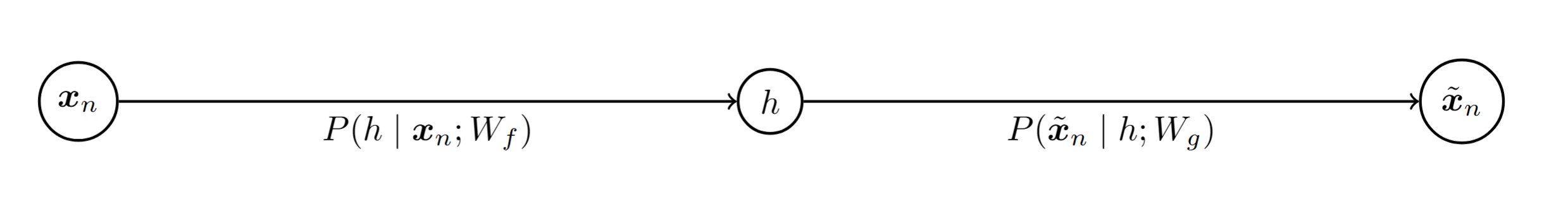
Variational autoencoders (VAEs) belong to a broader family of probabilistic autoencoders. Probabilistic autoencoders learn to model the distribution of the data in the latent space enabling them to generate new examples by sampling from this distribution. A VAE consists of an encoder and a decoder part. The encoder maps an input \(x\) to a distribution over the latent space, encoding it into a conditional distribution of latent variables rather than a single point. The decoder then samples from this latent distribution to produce a conditional distribution over possible reconstructions of \(x\). Denote these conditional distributions as \(f\) and \(g\) for the encoder and decoder, respectively. Then
- \(f: Pr(h \mid x; W_f)\), where \(h\) is the latent representation conditioned on the input \(x\), and \(W_f\) are the parameters of the encoder.
- \(g: Pr(\tilde{x} \mid h; W_g)\), where \(\tilde{x}\) is generated from the latent representation \(h\), with \(W_g\) as the parameters of the decoder.
The key idea in a VAEs is to ensure that the encoder distribution over the latent space is close to a simple, fixed distribution, typically a standard normal distribution \(\mathcal{N}(0, I)\). As a result, to generate new data points, we can easily sample new latent representations from \(\mathcal{N}(0, I)\) and pass them through the decoder.
So we have two simultaneous goals. First, to reconstruct \(x\) with high probability. Second, to ensure that \(\Pr(h \mid x; W_f)\) is close to \(\mathcal{N}(0, I)\). Denoting the training dataset by \(\{x_1,\cdots,x_m\}\), this leads to the following objective function:
\[\max_{W} \sum_{m} \log \Pr(x_n; W_f, W_g) - \beta \text{KL}\left(\Pr(h \mid x_n; W_f) \| \mathcal{N}(h; 0, I)\right)\]We have
\[\Pr(x_n; W_f, W_g) = \int_h \Pr(x_n \mid h; W_g) \Pr(h \mid x_n; W_f) dh\]In order to compute this integral, we make two simplifications:
- First, assume that
where the mean \(\mu_n\) and variance \(\sigma_n\) are obtained through the encoder. Therefore,
\[\Pr(x_n; W_f, W_g) = \int_h \Pr(x_n \mid h; W_g) \mathcal{N}(h; \mu_n(x_n; W_f), \sigma_n^2(x_n; W_f) I) dh\]- Second, approximate this integral by a single sample, namely:
NB: In the context of training with stochastic gradient descent, this may not be considered an oversimplification!
The figure below illustrates the network architecture.
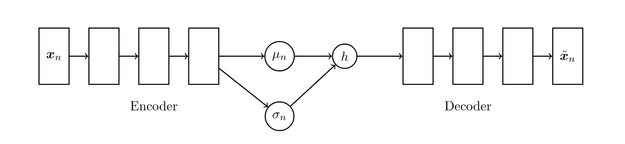
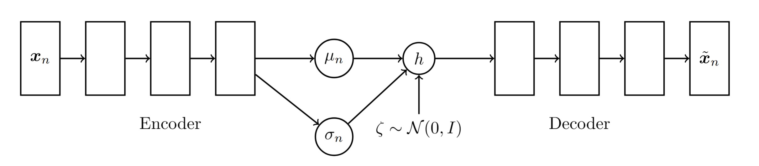
With this architecture, we face a challenge when trying to backpropagate through the stochastic sampling step. The sampling introduces randomness, which disrupts the flow of gradients and makes the training infeasible. To address this, VAEs use a technique called the reparameterization: Instead of sampling directly from the latent distribution \(h \sim q(h\\|x)\), we rewrite \(h\) as a deterministic function of the encoder’s output parameters and an independent random variable \(\zeta \sim N(0,I)\). The reparameterization trick transforms the sampling as follows:
\[h = \mu_n(x) + \sigma_n(x) \cdot \zeta \quad \text{where} \quad \zeta \sim \mathcal{N}(0,I)\]Here \(\mu_n(x)\) and \(\sigma_n(x)\) are the mean and standard deviation of the latent distribution \(q(h\\|x)\).
This transformation effectively makes the sample \(h\) a function of \(x\) and the learned parameters \(W_f\), with the randomness isolated in \(\zeta\). Now, \(h\) can be treated as a deterministic input to the decoder network during backpropagation, allowing us to compute gradients with respect to the encoder parameters. The resulting network looks as follows:
Now, returning to the second approximation (recal that \(Pr(x_n; W_f, W_g)\) represents the probability of reconstructing \(x_n\)), we have that:
\[\log Pr(x_n; W_f, W_g) \approx -\frac{1}{2}\Vert x_n-\tilde{x}_n\Vert^2\]Moreover, it is noted that the KL divergence between \(N(\mu, \sigma^2)\) and \(\mathcal{N}(0, 1)\) is given by:
\[D_{\text{KL}} \big( N(\mu, \sigma^2) \parallel \mathcal{N}(0, 1) \big) = \frac{1}{2} \left( \sigma^2 + \mu^2 - 1 - \ln(\sigma^2) \right)\]Putting pieces together and scaling by 2, we derive the following loss function for training our VAE:
\[\min \frac{1}{m}\sum_n \Vert x_n-\tilde{x}_n\Vert^2 + \frac{\beta}{m} \cdot \sum_n\left( \sigma_n^2 + \mu_n^2 - 1 - \ln(\sigma_n^2) \right)\]Two important notes are in order:
- \(\frac{1}{m}\sum_n \Vert x_n-\tilde{x}_n\Vert^2\) grows with \(\text{dim}(x_n)\). In other words, there is no normalization factor to take into account the input data point’s dimension.
- \(\mu_n\) and \(\sigma_n\) are functions of \(W_f\), the encoder’s weights. It is problem-specific how to choose the specifics of these functions. For example, in this project, we ask the network to learn \(\log \sigma\). In other words, \(\log \sigma = f_\sigma(W_f)\) for some function of \(W_f\).
Heston Model
Heston model consists of two coupled stochastic differential equations (SDEs):
\[\begin{align*} dS_t &= S_t \mu dt + S_t \sqrt{v_t} dW_t^S\\ dv_t &= \kappa (\theta - v_t) dt + \sigma \sqrt{v_t} dW_t^v \end{align*}\]| Symbol | Description |
|---|---|
| \(S_t\) | The asset price at time \(t\) |
| \(\mu\) | The drift rate i.e., expected return |
| \(v_t\) | The variance at time \(t\) |
| \(\kappa\) | The rate of mean reversion |
| \(\theta\) | The long-term variance i.e., mean reversion level |
| \(\sigma\) | The volatility of volatility i.e., how much \(v_t\) fluctuates |
| \(W_t^S, W_t^v\) | Wiener processes where \(d W_t^S d W_t^v = \rho dt\) |
Training Data
The following sets of maturities and log-moneyness are considered for our European options. The maturities in days are defined as:
\[\tau_{\text{days}} = \{6, 12, 18\} \cup \{26 \cdot x \mid x \in \{1, 2, \ldots, 14\}\}.\]The set of log-moneyness values, \(k_{\text{aux}}\), is constructed as follows. Let:
\[x_{\min} = -k_{\min}^{1/3}, \quad x_{\max} = k_{\max}^{1/3},\]where \(k_{\min} = 0.4\) and \(k_{\max} = 0.6\). Then:
\[k_{\text{aux}} = \{x^3 \mid x \in \text{linspace}(x_{\min}, x_{\max}, 100)\}.\]It is emphasized that this construction ensures that more log-moneyness values are concentrated around at-the-money (ATM) levels.
Next, we define a set of values for the Heston parameters. We fix \(v_0 = 0.05, \mu = r = q = 0\), and spot = 1. For the remaining four parameters \(\kappa, \eta, \rho\), and \(\sigma\), we consider a range for each and divide it into \(n_{\text{steps}} = 5\) equally spaced intervals. This results in \(n_{\text{steps}}^4 = 625\) possible combinations of parameter values. The table below shows the considered ranges.
| Parameter | Range | Steps |
|---|---|---|
| \(\kappa\) | From 0.1 to 0.9 | 5 |
| \(\eta\) | From \(0.05^2\) to \(0.25^2\) | 5 |
| \(\rho\) | From -0.9 to -0.1 | 5 |
| \(\sigma\) | From 0.1 to 0.5 | 5 |
Monte Carlo Simulation
We now try to generate a set of 625 volatility surfaces. Monte Carlo simulation with the Full Truncation method is used to compute option prices under these 625 Heston parameter combinations. The pricing code is implemented in PyTorch to leverage GPU acceleration. To handle the computational load, \(2^{\text{num-path-log}}\) Monte Carlo paths are generated in multiple rounds, and the resulting prices are averaged. This approach mitigates potential issues such as GPU memory exhaustion, which can lead to reduced speed or memory errors. You can adjust the number of paths and rounds based on your available computational resources.
Once the option prices are calculated, we use QuantLib to compute the corresponding implied volatilities. Note that, initially, we consider the full grid of \((k, \tau)\) values, where \(k \in k_{\text{aux}}\) and \(\tau \in \tau_{\text{days}}\). However, implied volatility is not successfully computed for all these grid points. To address this issue, we retain only those grid points (which happen to form a triangular shape) at which the implied volatility is successfully calculated for all 625 processes.
num_path_log = 23
round_log = 0
num_paths = 2**num_path_log

def pricing(kappa,eta,rho,sigma):

    kappa_dt = torch.tensor(kappa * dt)
    sdt = torch.sqrt(torch.tensor(dt, dtype=torch.float64,device=device))
    df_gpus = []

    for _ in range(2**round_log):

        df_gpu = pd.DataFrame(index=taus_days[1:], columns=K_aux)
        stocks = {t: [] for t in taus_days[1:]}
        S = torch.full((num_paths,), spot, dtype=torch.float64, device=device)  # Initial asset price
        v = torch.full((num_paths,), v0, dtype=torch.float64, device=device)  # Initial variance
        for t in range(1, timesteps + 1):

            Zs = torch.randn(num_paths,  dtype=torch.float64, device=device)
            Z1 = torch.randn(num_paths,  dtype=torch.float64, device=device)

            vol = torch.sqrt(torch.relu(v))
            volsigma = vol*sigma

            v = v + kappa_dt * (eta - torch.relu(v)) + volsigma*sdt * (rho * Zs - torch.sqrt(1 - rho**2) * Z1)
            S = S * torch.exp((- 0.5 * vol**2) * dt + vol*sdt * Zs)

            if t in taus_days[1:]:
                stocks[t].append(S)

        for t in taus_days[1:]:
            stocks[t] = torch.cat(stocks[t],dim=0)

        stocks_tensor = torch.stack([stocks[t] for t in taus_days[1:]], dim=0)
        del stocks
        for strike in K_aux: df_gpu.loc[:, strike] = torch.relu(stocks_tensor-strike).mean(axis=1).cpu()
        df_gpus.append(df_gpu)

    df_av = sum(df_gpus)/len(df_gpus)


    ### Computing the implied volatility

    ivs = pd.DataFrame(index=taus_days[1:], columns=K_aux)
    for tau_idx, tau_day in enumerate(taus_days[1:]):

        tau = Times[tau_day]
        expiry_date = today+ql.Period(tau_day,ql.Days)

        for strike_idx, strike in enumerate(K_aux):

            option_price = df_av.iloc[tau_idx, strike_idx]
            iv = quantlib_iv(tau,strike, spot, float(r),float(q),today,expiry_date,option_price)
            ivs.loc[tau_day, strike] = iv

    # 0.05 was the lower bound considered for Quantliv IV calucation.
    ivs[ivs==0.05] = np.nan

    # return df_av, ivs
    return ivs
The VAE Model Training
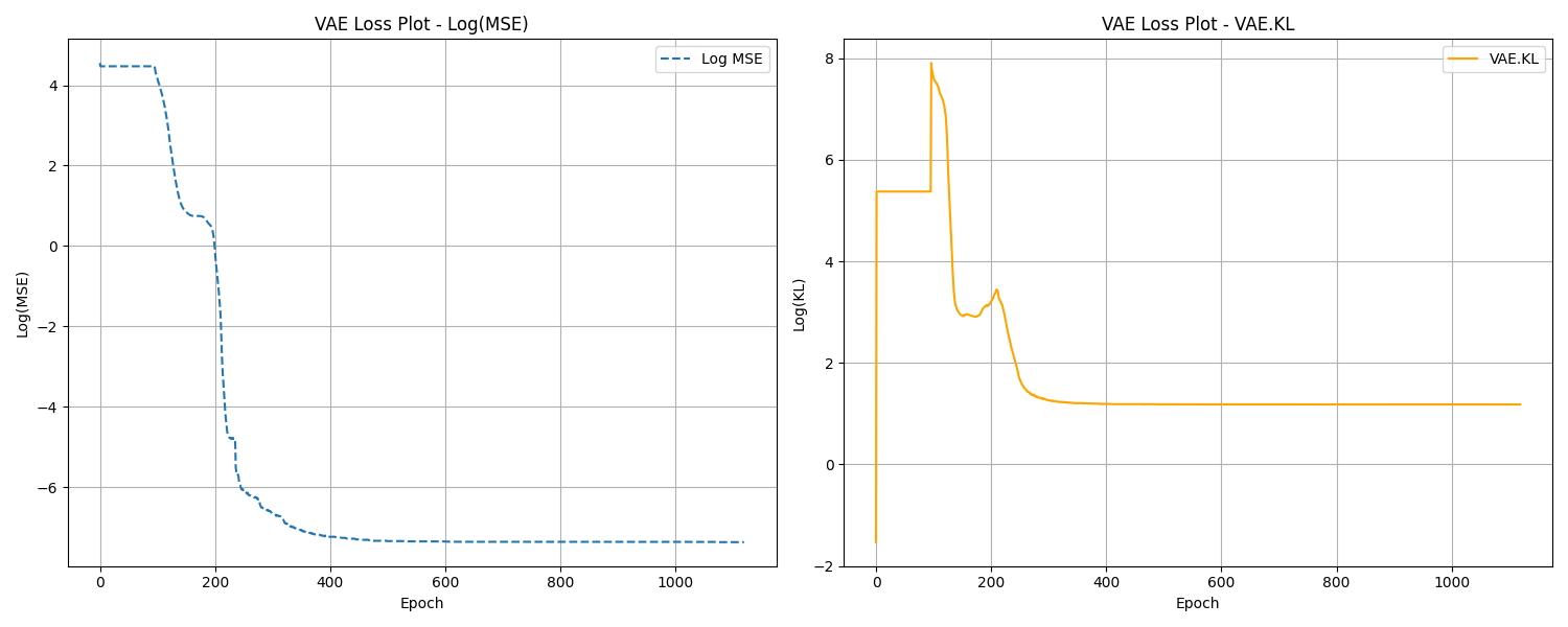
Python code below shows how the VAE module is constructed and trained! As discussed earlier, the loss function comprises two components: the Mean Squared Error (MSE) loss and the KL divergence loss. The total loss is defined using the constant \(\beta\) parameter, and the two components of the loss are recorded whenever the best total loss value is identified during training.
It is emphsized that during training, the MSE loss converges to zero while the KL divergence loss levels off at 3. While this may not be optimal, it is sufficient for the purposes of our generative model.
hidden_sizes_encoder = [32, 64,128]
hidden_sizes_decoder = [dim for dim in reversed(hidden_sizes_encoder)]
latent_dims = 4

class Encoder(nn.Module):

    def __init__(self, hidden_sizes_encoder, latent_dims):

        super(Encoder, self).__init__()
        layers = []
        in_size = training_data.shape[1]
        for hidden_size in hidden_sizes_encoder:
            layers.append(nn.Linear(in_size, hidden_size).to(torch.float64))
            layers.append(nn.LeakyReLU())
            in_size = hidden_size
        self.layer_mu = nn.Linear(in_size, latent_dims).to(torch.float64)
        self.layer_var = nn.Linear(in_size, latent_dims).to(torch.float64)
        self.network = nn.Sequential(*layers)

    def forward(self, x):
        x = self.network(x)
        mu =  self.layer_mu(x)
        log_var = self.layer_var(x)
        std = torch.exp(0.5 * log_var)
        eps = torch.randn_like(std)
        z = eps * std + mu #torch.Size([625, 4])
        self.kl = 0.5*(mu ** 2 + log_var.exp()-1 - log_var).mean()

        return z

class Decoder(nn.Module):

    def __init__(self, hidden_sizes_decoder, latent_dims):
        super(Decoder, self).__init__()
        layers = []
        in_size = latent_dims
        layers.append(nn.Linear(in_size, hidden_sizes_decoder[0]).to(torch.float64))

        for i in range(len(hidden_sizes_decoder)-1):

            dim_1, dim_2 = hidden_sizes_decoder[i],hidden_sizes_decoder[i+1]
            layers.append(nn.Linear(dim_1, dim_2).to(torch.float64))
            layers.append(nn.LeakyReLU())

        layers.append(nn.Linear(hidden_sizes_decoder[-1], training_data.shape[1]).to(torch.float64))
        layers.append(nn.LeakyReLU())

        self.network = nn.Sequential(*layers)

    def forward(self, x):
        return self.network(x)


class VariationalAutoencoder(nn.Module):

    def __init__(self, hidden_sizes_encoder, hidden_sizes_decoder, latent_dims):

        super(VariationalAutoencoder, self).__init__()
        self.encoder = Encoder(hidden_sizes_encoder, latent_dims)
        self.decoder = Decoder(hidden_sizes_decoder, latent_dims)

    def forward(self, x):
        z = self.encoder(x)
        return self.decoder(z)

print_epoch = 1000
print(f'Print every {print_epoch} epochs!')
def train(autoencoder, epochs=print_epoch*10000):

    best_loss = float('inf')
    kl_saved = float('inf')
    mse_saved = float('inf')
    header_message = f"{'Epoch':>5} | {'Cur LR':>20} | {'Cur MSE':>20} | {'Cur KL':>20} | {'Saved KL':>20} | {'Saved MSE':>20} | {'KL Reg':>20}"

    print(header_message)
    opt = torch.optim.Adam(autoencoder.parameters(), lr=0.01,weight_decay=0.01)
    scheduler = optim.lr_scheduler.ReduceLROnPlateau(opt, mode='min', factor=0.9, patience=3*print_epoch, min_lr=1e-6)
    epoch = 0
    beta = 1
    while best_loss > 1e-5 and epoch <epochs:

        opt.zero_grad()
        iv_stacked_hat = autoencoder(training_data)
        loss_mse_ = F.mse_loss(iv_stacked_hat, training_data)
        loss_mse =  loss_mse_*training_data.shape[1]
        kl = autoencoder.encoder.kl
        loss = loss_mse+beta*kl
        loss.backward()
        opt.step()
        cur_lr = opt.state_dict()["param_groups"][0]["lr"]
        total_loss =  loss_mse + beta*kl
        scheduler.step(total_loss)

     if best_loss > loss.item():

            best_loss = loss.item()
            mse_saved = loss_mse_.item()
            kl_saved = kl.item()
            torch.save(autoencoder.state_dict(), 'autoencoder.pth')

        if epoch % print_epoch == 0:
            print(f"{int(epoch/print_epoch):>5} | {cur_lr:>20.10f} | {loss_mse_.item():>20.10f} | {kl.item():>20.10f} | {kl_saved:>20.10f} | {mse_saved:>20.10f} | {beta:>20.10f}")

        epoch = epoch + 1
    return autoencoder
The figure below displays the logarithmic values of the MSE and KL divergence losses during the training process.
Generative VAE model for Heston Model
Once the VAE model is trained, we use it to generate new volatility surfaces in two different ways:
- Random walk in laten space: Create a family of Heston volatility surfaces by using a random walk in the latent space of the Heston model.
- Fitting randomly generated surfaces: Test the VAE’s capability to generate a volatility surface that closely fits a randomly generated target surface. This involves optimizing within the latent space to minimize the difference between the VAE-generated surface and the target surface.
The next two subsections provide detailed explanations of these approaches.
Random Walk
To explore the generative capabilities of my Variational Autoencoder (VAE), I create a random walk in \(R^{\text{latent dim}}\). This random walk is generated using Gaussian steps with their length re-scaled to \(dt=0.2\). The resulting random walk serves as the input trajectory to the VAE. The GIF below displays a walk of size 500. Right click on the GIF and ‘Open in new tab’ if the GIF doesn’t display the animation.
Fit a Random Surface Using the VAE Model
We next evaluate the generalization capabilities of our VAE model. To achieve this, we generate a random set of parameters and compute option prices through Monte Carlo simulations. Using these prices, we derive the implied volatility surface with the help of the QuantLib library. Subsequently, we employ the Adam optimizer to identify a point in the latent space that, when processed through the VAE, generates a volatility surface closely approximating the target surface, as measured by the mean squared error (MSE) loss. The Python snippet below shows the process.
from gen_training import pricing

### Generate a random Heston Volatility Surface

kappa_min, kappa_max = 0.1, 0.9
eta_min, eta_max = 0.05**2, 0.25**2
rho_min, rho_max = -0.9, -0.1
sigma_min, sigma_max = 0.1, 0.5


kappa_random = torch.empty(1).uniform_(kappa_min, kappa_max).to(device)
eta_random = torch.empty(1).uniform_(eta_min, eta_max).to(device)
rho_random = torch.empty(1).uniform_(rho_min, rho_max).to(device)
sigma_random = torch.empty(1).uniform_(sigma_min, sigma_max).to(device)

random_prices = pricing(kappa_random,eta_random,rho_random,sigma_random)
random_prices = (random_prices*random_prices).mul(random_prices.index, axis=0)
random_array = (random_prices*no_nan_mask_df).replace(0, np.nan).values
random_tensor = torch.tensor(random_array[~np.isnan(random_array)]).to(device)


### Load VAE model

hidden_sizes_encoder = [32, 64,128]
hidden_sizes_decoder = [dim for dim in reversed(hidden_sizes_encoder)]
latent_dims = 4
vae = VariationalAutoencoder(hidden_sizes_encoder, hidden_sizes_decoder, latent_dims).to(device)
vae.load_state_dict(torch.load('autoencoder.pth'))

### Track gradients when search through the latent space

class GDModel(nn.Module):
    def __init__(self):
        super(GDModel, self).__init__()
        self.linear = nn.Linear(1,latent_dims).to(torch.float64)

    def forward(self):
        # import pdb; pdb.set_trace()
        out = self.linear(torch.tensor([1.0]).to(torch.float64).to(device))
        return out

vae.eval()
best_loss = float('inf')
epoch = 0

### Using Adam to find a point in the latent space that produces a similar volatility surface when passed through the VAE

gdmodel = GDModel().to(device)
optimizer = optim.Adam(gdmodel.parameters(), lr=0.1)
scheduler_args = {'mode':'min', 'factor':0.9, 'patience':100, 'threshold':0.05}
scheduler = optim.lr_scheduler.ReduceLROnPlateau(optimizer, **scheduler_args)

losses = []
num_epochs  = 50000
with torch.no_grad():
    fit_vae = vae.decoder(gdmodel())

while epoch < num_epochs:

    optimizer.zero_grad()
    loss = F.mse_loss(vae.decoder(gdmodel()),random_tensor)
    loss.backward()
    optimizer.step()
    # scheduler.step(loss)
    if loss < best_loss:
        best_loss = loss
        print(best_loss.item())
        with torch.no_grad():
            fit_vae = vae.decoder(gdmodel())
    cur_lr = optimizer.state_dict()["param_groups"][0]["lr"]
    losses.append(loss.item())
    epoch += 1

## plot(fit_vae & random_tensor)
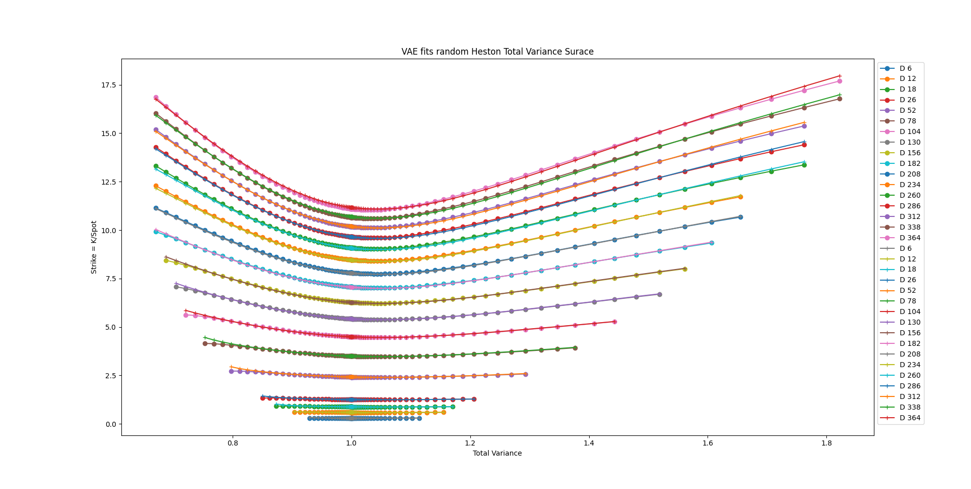
Figure below is an example of VAE’s capablity of fitting a random surface. The ‘o’ marker represents the VAE’s output.
Bibtex
@misc{baghal2024generative,
  title={Generative Modeling of Heston Volatility Surfaces Using Variational Autoencoders},
  author={Baghal, Sina},
  journal={https://sinabaghal.github.io/vae4heston/},
  url={https://sinabaghal.github.io/vae4heston/},
  year={2024}
}
The full source code for this project is available at here.
References
Kingma, D., Welling, M. (2019). An Introduction to Variational Autoencoders. arXiv:1906.02691 ↩
Poupart, P. (2019). Introduction to Machine Learning. CS480/690 UWaterloo ↩