
Basics of Reinforcement Learning
This tutorial provides an introduction to the fundamentals of reinforcement learning. The main reference is the video lecture series by Sergey Levine. Read the PDF version here.
Table of Contents
What is RL?
RL: In reinforcement learning, there is an agent and an environment. At time step \(t\), the state is denoted by \(s_t\). Given state \(s_t\), the agent takes an action \(a_t\) resulting in a reward value \(r_t := r(s_t, a_t)\).
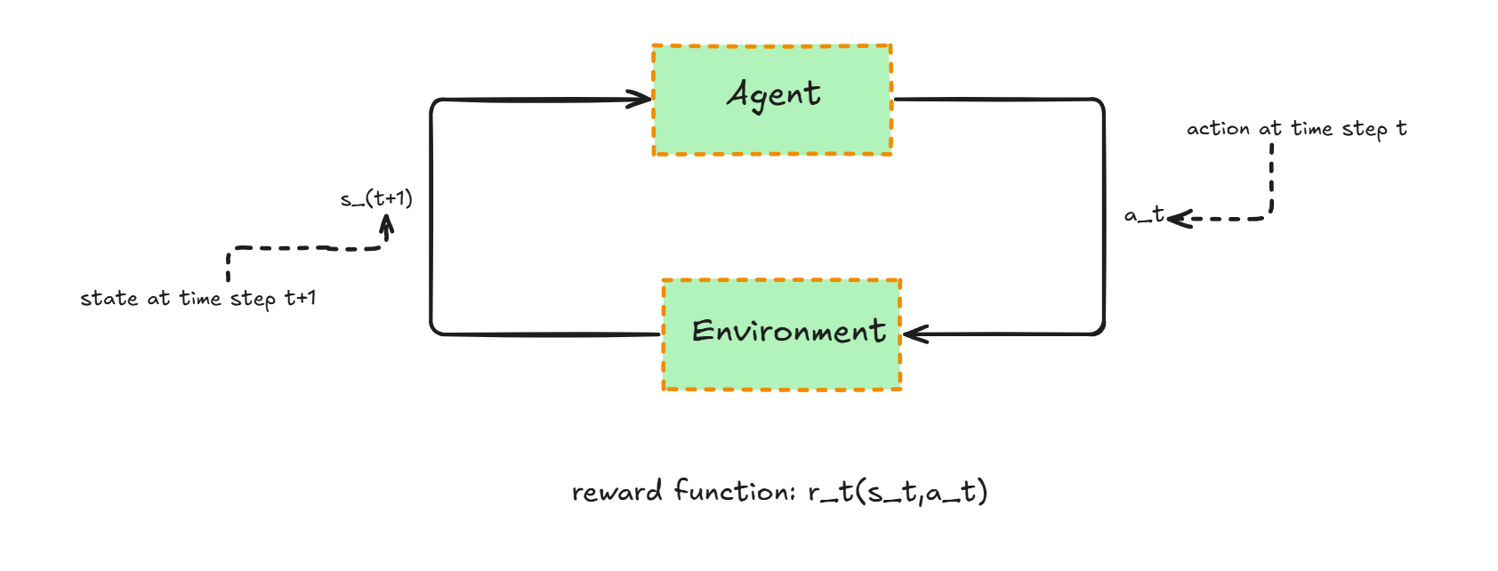
Policy: The agent’s policy is parameterized by \(\pi_\theta\), where \(\pi_\theta(\cdot \mid s_t)\) defines a probability distribution over possible actions at time \(t\), given the state \(s_t\).
RL Goal: The goal of an RL algorithm is to maximize the expected cumulative reward:
\[\text{argmax}_\theta \; \mathbb{E}_{\pi_\theta} \left[ \sum_{t=0}^T \gamma^t r(s_t, a_t) \right],\]where \(0 \leq \gamma < 1\) and \(T\) are the discount factor and horizon respectively. Notice that:
- More weight is placed on earlier steps.
- \(\mathbb{E}_{\pi_\theta}\) is a smooth function of \(\theta\) where \(r\) itself may not be (e.g., \(r \in \{\pm 1\}\)).
- \(s_t\) is independent of \(s_{t-1}\) (Markov Property).
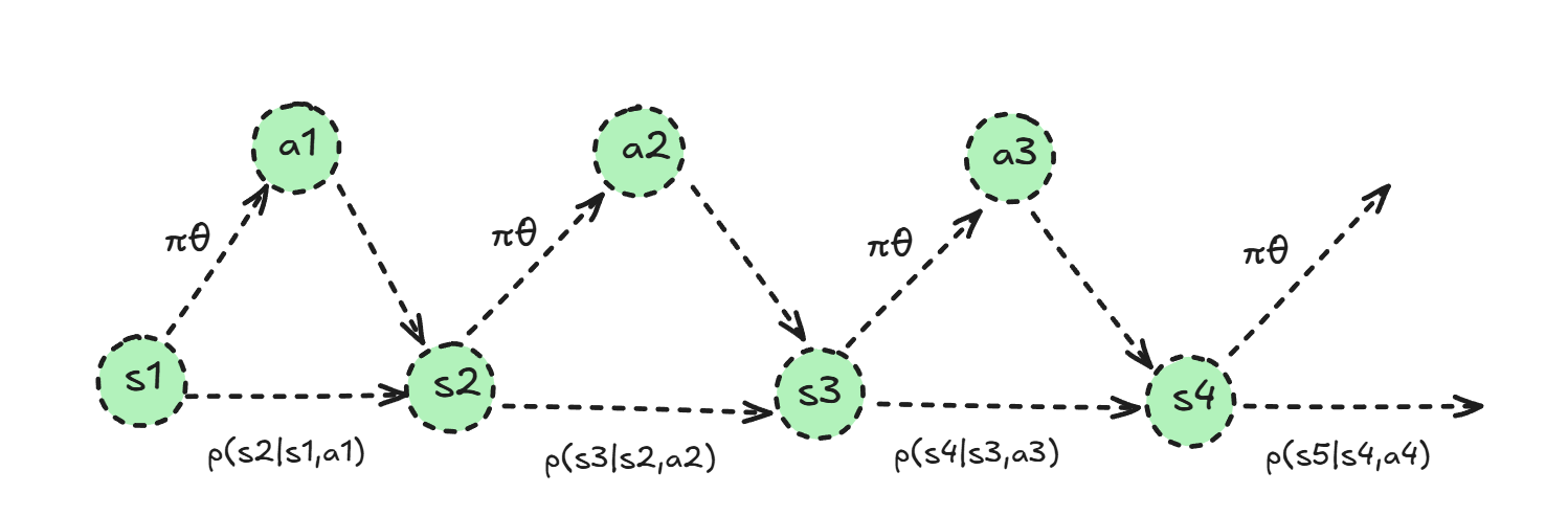
MDP: A Markov Decision Process (MDP) consists of a state space \(\mathcal{S}\) and an action space \(\mathcal{A}\), along with a transition operator \(\mathcal{T}\) and a reward function \(r : \mathcal{S} \times \mathcal{A} \to \mathbb{R}_+\). An MDP allows us to write a probability distribution over trajectories:
\[p_\theta(\tau) = p(s_1)\prod_{t=1}^T \pi_\theta(a_t|s_t)p(s_{t+1}|s_t,a_t), \quad \text{where } \tau = (s_1,a_1,\dots,s_T,a_T).\]Imitation Learning
The analogous concept in reinforcement learning, compared to supervised learning, is called imitation learning, where the agent learns by mimicking expert actions. However, imitation learning often does not work well in practice due to the distributional shift problem. This arises because, in supervised learning, samples are assumed to be i.i.d., while in reinforcement learning the agent’s past actions affect future states.
Assume that $\pi^*$ is the expert policy and the learned policy $\pi_\theta$ makes an error with probability at most $\epsilon$ under the training distribution:
\[\Pr_{s_t \sim p_{\text{train}}}\big[\pi_\theta(s_t) \neq \pi^*(s_t)\big] \leq \epsilon.\]Then,
\[p_{\theta}(s_t) = (1-\epsilon)^t p_{\text{train}}(s_t)+(1-(1-\epsilon)^t)p_{\text{mistake}}(s_t).\]Denote \(c_t(s_t, a_t) = 1_{\{a_t \neq \pi^*(s_t)\}} \in \{0, 1\}\). Then the total number of times the policy \(\pi_\theta\) deviates from the optimal policy grows quadratically with \(T\):
\[\begin{aligned} \mathbb{E}_{\pi_\theta} \left[ \sum_{t=0}^T c(s_t,a_t) \right] &= \sum_{t=0}^T\int p_\theta(s_t)c(s_t,a_t) ds_t \\ &= \sum_{t=0}^T (1-\epsilon)^t\int p_{\text{train}}(s_t)c(s_t,a_t) ds_t + \sum_{t=0}^T (1-(1-\epsilon)^t)\int p_{\text{mistake}}(s_t)c(s_t,a_t) ds_t \\ &\leq \sum_{t=0}^T (1-\epsilon)^t\epsilon + \sum_{t=0}^T 1-(1-\epsilon)^t \\ &\leq \sum_{t=0}^T (1-\epsilon)^t\epsilon + 2\epsilon\sum_{t=0}^T t \\ &= \epsilon\cdot\mathcal{O}(T^2) \end{aligned}\]This bound is achieved in the tightrope walking problem, where the agent must learn to go straight; otherwise, it will enter unknown territory. Imitation learning can still be useful with some modifications, such as including bad actions along with corrective steps.

REINFORCE
An MDP allows us to rewrite the goal of RL as the following optimization problem:
\[\text{argmax}_\theta \; J(\theta):= \mathbb{E}_{\tau \sim p_\theta}[r(\tau)] = \int p_\theta(\tau)r(\tau)d\tau,\]enabling a direct policy differentiation:
\[\begin{aligned} \nabla_\theta J(\theta) &= \int \nabla_\theta p_\theta(\tau)r(\tau)d\tau \\ &= \int p_\theta(\tau)\nabla_\theta \log p_\theta(\tau)r(\tau)d\tau \\ &= \mathbb{E}_{\tau \sim p_\theta} \nabla_\theta \log p_\theta(\tau)r(\tau) \\ &= \mathbb{E}_{\tau \sim p_\theta} \left(\sum_{t=1}^T \nabla_\theta \log \pi_\theta(a_t|s_t)\right)\cdot\left(\sum_{t=1}^T r(s_t,a_t)\right) \end{aligned}\]REINFORCE Algorithm:
Run the current policy \(N\) times to generate sample \(\tau_i$ for $i=1,\dots,N\).
Compute the Monte Carlo estimate:
- Apply Gradient Ascent: \(\theta \leftarrow \theta + \alpha \nabla_\theta J(\theta)\).
Variance Reduction
One of the main issues with REINFORCE is the high variance in the reward term \(\sum_{t=1}^T r(s_{i,t},a_{i,t})\). In this section, we introduce some techniques to reduce this variance.
Causality
As a first step toward variance reduction, we apply the causality trick:
Policy at time \(t'\) cannot impact reward at time \(t < t'\).
Using this, the policy gradient is estimated as:
\[\nabla_\theta J(\theta) \approx \frac{1}{N}\sum_{i=1}^N \sum_{t=1}^T \nabla_\theta \log \pi_\theta(a_{i,t}|s_{i,t}) \left(\sum_{t'=t}^T r(s_{i,t'},a_{i,t'})\right)\]The term \(\sum_{t'=t}^T r(s_{i,t'},a_{i,t'})\) is referred to as the reward-to-go.
Value Functions
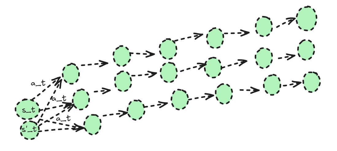
The next idea is to replace the reward-to-go with a function estimator. Notice two things: the ideal target for the reward-to-go function is
\[Q(s_{i,t},a_{i,t}) = \sum_{t'=t}^T\mathbb{E}_{\pi_{\theta}}[r(s_{t'},a_{t'})|s_{i,t}, a_{i,t}]\]| rather than the single-sample estimate \(\sum_{t'=t}^T r(s_{i,t'},a_{i,t'})\). This represents the value of state $s_{i,t}$ under the current policy where action $a_{i,t}$ is taken. Another advantage is that, as shown in Figure below, if the state \(s′_{i,t}\) is quite close to \(s'_{i,t}\) and $$p(s_{t+1} | s’{i,t},a’{i,t})\approx p(s_{t+1} | s_{i,t},a_{i,t})$$, we expect their reward-to-go values to be similar. However, when working with a single-sample estimate, this relationship may easily be violated. |
Baselines
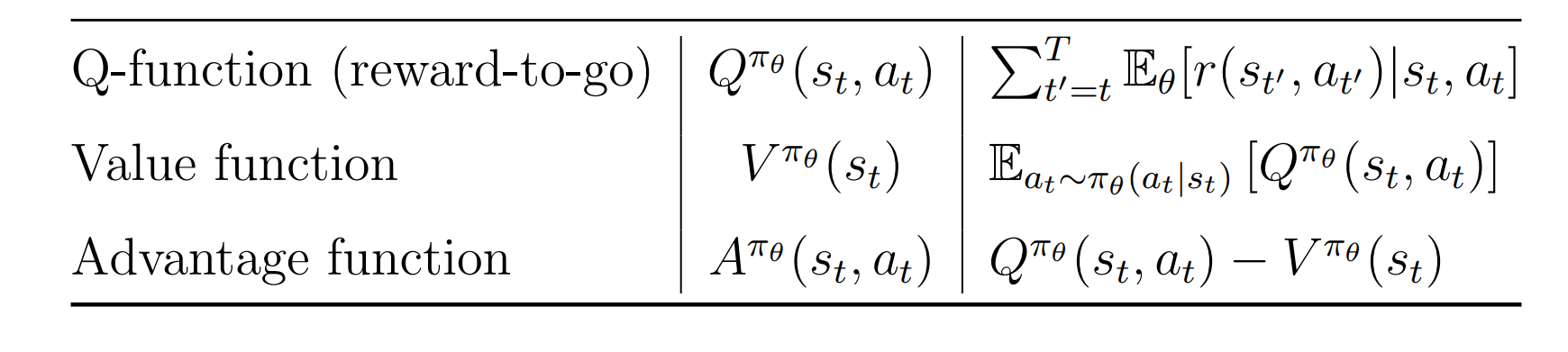
Translation of the reward \(r \mapsto r - b\) can help reduce variance. Assuming this translation:
\[\begin{aligned} \text{Var}[\nabla_\theta J(\theta)] &= \mathbb{E}_{\tau \sim p_\theta(\tau)} \left(\nabla_\theta \log p_\theta(\tau)(r(\tau)-b)\right)^2- \left(\mathbb{E}_{\tau \sim p_\theta(\tau)}\nabla_\theta \log p_\theta(\tau)(r(\tau)-b)\right)^2\\ &= \mathbb{E}_{\tau \sim p_\theta(\tau)} \left(\nabla_\theta \log p_\theta(\tau)(r(\tau)-b)\right)^2-\left(\mathbb{E}_{\tau \sim p_\theta(\tau)}\nabla_\theta \log p_\theta(\tau)r(\tau)\right)^2 \end{aligned}\]Thus, an appropriate choice of $b$ can reduce the variance. A proper choice is the expected value of the $Q$ function. Table below summarizes value functions used throughout.
Thus following policy gradient favors lower variance:
\[\nabla_\theta J(\theta) = \mathbb{E}_{\tau \sim p_\theta}\sum_{t=1}^T \nabla_\theta \log \pi_\theta(a_t|s_t) \cdot \left[r(s_t,a_t)+V^{\pi_\theta}(s_{t+1})-V^{\pi_\theta}(s_{t})\right]\]Discounts
The discount factor also helps reduce variance, as terms further in the horizon are weighted less. The policy gradient becomes:
\[\nabla_\theta J(\theta) = \mathbb{E}_{\tau \sim p_\theta}\sum_{t=1}^T \nabla_\theta \log \pi_\theta(a_t|s_t) \cdot \left[r(s_t,a_t)+\gamma \hat{V}_\phi^{\pi_\theta}(s_{t+1})-\hat{V}_\phi^{\pi_\theta}(s_{t})\right]\]Here $\hat{V}_\phi$ estimates $V$.
Bias Reduction
The policy gradient derived in the previous section, while enjoying low variance, is prone to higher bias.
We tune this bias-variance trade-off using the $n$-step return estimator:
For $n=1$, we recover the previously mentioned policy gradient. As $n \to +\infty$, the bias is reduced while the variance increases. To manage this trade-off, we define the Generalized Advantage Estimator (GAE):
\[\begin{aligned} \hat{A}^{\pi_\theta}_{GAE} &= \sum_{n=1}^{+\infty} \lambda^{n-1} \hat{A}^{\pi_\theta}_n \\ &= \sum_{t'=t}^{+\infty} (\gamma \lambda)^{t'-1} \delta_{t'} , \quad \delta_{t'} = r(s_{t'},a_{t'}) + \gamma \hat{V}_\phi(s_{t'+1}) - \hat{V}_\phi(s_{t'}) \end{aligned}\]The final policy gradient is then:
\[\nabla_\theta J(\theta) = \mathbb{E}_{\tau \sim p_\theta} \sum_{t=1}^T \nabla_\theta \log \pi_\theta(a_t|s_t) \cdot \hat{A}^{\pi_\theta}_{GAE}(s_t,a_t)\]